Model Quantization

Model Compression

The process of making a model smaller is called model compression, and the process to make it do inference faster is called inference optimization.

Low-Rank Factorization (The key idea behind low-rank factorization is to replace high-dimensional tensors with lower-dimensional tensors)
Knowledge Distillation (Knowledge distillation is a method in which a small model (student) is trained to mimic a larger model or ensemble of models (teacher). The smaller model is what you’ll deploy. Even though the student is often trained after a pretrained teacher, both may also be trained at the same time.)
Pruning (Pruning was a method originally used for decision trees where you remove sections of a tree that are uncritical and redundant for classification.25 As neural networks gained wider adoption, people started to realize that neural networks are over parameterized and began to find ways to reduce the workload caused by the extra parameters.)
Quantization (Quantization reduces a model’s size by using fewer bits to represent its parameters.)

Quantization

Quantization is a technique used to reduce the memory footprint and computational requirements of LLMs, particularly when dealing with limited hardware resources.

Conversion Process: Quantization involves converting model parameters, typically stored as 32-bit floating point numbers (FP32), to lower precision formats like 8-bit integers (INT8) or 16-bit floating point numbers (FP16).

Overcoming Accuracy Loss: Techniques like quantization-aware training (QAT) help mitigate accuracy loss by fine-tuning the quantized model with additional training data.

Symmetric vs. Asymmetric Quantization:

Symmetric quantization, like batch normalization, centers the data distribution around zero (mean the value start from 0 instead of negative)
Asymmetric quantization utilizes a zero-point to handle data distributions that are not symmetrical (vaule may have a negative value)

Process of Symmetric:

Identify the minimum and maximum values (xmin and xmax) within the weight data.
Determine the quantization range: This is the difference between the maximum quantized value (Qmax) and the minimum quantized value (Qmin). For unsigned INT8, the range is 0 to 255.
Calculate the scale factor: This factor determines how the original floating-point values are mapped onto the quantized integer range. The formula for the scale factor is: scale = (xmax - xmin) / (Qmax - Qmin)
Quantize each weight value:
- Divide the weight by the scale factor. - Round the result to the nearest integer.
Example: converting floating-point numbers between 0 and 1000 to unsigned INT8. The scale factor is calculated as 3.92 (1000 / 255). A value of 250 would be quantized to 64 (250 / 3.92, rounded).
Process of Asymmetric:
- Identify xmin and xmax.
- Determine Qmax and Qmin.
- Calculate the scale factor: The formula remains the same as in symmetric quantization.
- Determine the zero-point: The zero-point represents the quantized value that corresponds to the original floating-point value of zero. The formula is: zero_point = Qmin - round(xmin / scale)
- Quantize each weight value:
  - Divide the weight by the scale factor.
  - Add the zero-point.
  - Round the result to the nearest integer.
Example: asymmetric quantization with a range of -20.0 to 1000. The scale factor is 4.0, and the zero-point is 5. The value of -20.0 is quantized to 0 (-20.0 / 4.0 + 5, rounded).

Modes of Quantization

post-training quantization (PTQ)
quantization-aware training (QAT)

PTQ

PTQ is applied after a model has been fully trained. It involves calibrating the model weights to determine appropriate scaling factors and zero-points, and then converting the weights from a higher precision format to a lower one
Theres is chance for loss of data

QAT

QAT incorporates quantization during the training process. It modifies the training procedure to make the model aware of the quantization that will occur later. This allows the model to adjust its weights to minimize the impact of quantization on its performance

Resource

A Visual Guide to Quantization

Types

AWQ: Activation-aware Weight Quantization for LLM Compression and Acceleration
- Efficient and accurate low-bit weight quantization (INT3/4) for LLMs, supporting instruction-tuned models and multi-modal LMs.
SqueezeLLM is a post-training quantization framework that incorporates a new method called Dense-and-Sparse Quantization to enable efficient LLM serving.

Example

Imagine you’re trying to send a big number to your friend over a walkie-talkie, but you can only use small numbers (like from -7 to 7). You need a way to shrink the big number to fit in that small range, and then later your friend needs a way to stretch it back.

That’s what quantization does:
🔹 Shrinks big floating-point numbers (like 3.14159) into small integers (like 3).
🔹 Later, we stretch it back to something close to the original.

Formula

Q = round(r / s - z)

Q is the quantized number (small integer)
r is the real float number
s is the scale (how much to shrink)
z is the zero point (like a shift to help line things up)

Let say You decide your real numbers go from -5.0 to 5.0 (your clipping range)

s = (max_real - min_real) / (max_int - min_int)
  = (5 - (-5)) / (7 - (-7))
  = 10 / 14 = 0.714

// to represent 3.4
Q = round(r / s) = round(3.4 / 0.714) ≈ round(4.76) = 5

we’re doing symmetric quantization, we can set z = 0.

Dequantization back

R_approx = (Q + z) * s
         = (5 + 0) * 0.714 = 3.57

How do we know to pick -5 to 5 for our real numbers?

This is called calibration. You run your model on a sample dataset and measure:

What’s the smallest value? (e.g., -4.8)
What’s the largest value? (e.g., 4.9)

Types

Legacy Quants (Oldest)

Type 0: Simple, assumes numbers are symmetric around zero. (symentric)
Type 1: More accurate, uses a “zero point” to shift the range.
Uses block quantization (like compressing groups of 16 or 32 numbers together).

Type 0 Example

We have 4 float numbers:

`[-1.2, -0.6, 0.2, 1.0]`

We want to fit them into 4-bit signed integers.

A 4-bit signed integer can represent:

`[-8, -7, ..., 0, ..., +7]`

That’s **15 values total**, and they’re **symmetric around 0**: `-7  -6  -5 ... 0 ... +5 +6 +7`

So **symmetric around 0** just means:

The smallest number is negative, the biggest is positive, and both have the same distance from 0.

K-Quants (Smarter Blocks)

Adds double compression: it compresses the weights and the constants (scale values).
Groups 8 blocks into a super block.
Less memory needed, faster to read.

This improves memory efficiency by compressing not only the weights but also the scales and offsets!

I-Quants (Vector Quantization)

Treats groups of weights as vectors (like arrows in space).
Matches these to reference vectors in a codebook.
Stores only the “closest match” plus some info.

Instead of quantizing each number or block, you treat a group of numbers as a vector. You then match this vector to a list of “known shapes” (codebook).

Suppose you have a vector of 8 weights:

W = [0.12, -0.55, 0.30, -0.71, ..., 0.20]

You have a codebook of 256 predefined vectors (called reference vectors), each 8-dimensional. It’s like saying:

“Which known shape is this vector closest to?”

You find the closest match using cosine similarity or Euclidean distance.

Then:

Store the code (e.g., code #76)
Store a scale so the matched vector is stretched to the correct magnitude
If needed, store sign bits for negative values

Dequantization:

Fetch the reference vector #76
Multiply it by the stored scale
Flip signs back using sign bits

Dequantize

We store the number in 4bit or 8bit but when we do the multilplication or any other operation we need to get back to the original vaule for that we have formula of

Q3=round(

((s1 - s2 / s3) * (Q1-Z1) * (Q2-Z2)) + Z3

)

Q1,Q2 are the quantized values (integers) of the input floats.
s1,s2,s3s_1, s_2, s_3s1,s2,s3 are the scales for the inputs and output. (the scale fator may change for because when we do quantize we pick bathc of number under one range etc)
z1,z2,z3z_1, z_2, z_3z1,z2,z3 are the zero points for the inputs and output.
The rounding function is used to ensure the result stays an integer.


r1 = 2.0
r2 = 1.5 
r3 = r1 * r2 = 3.0


same in quantization
s1 = s2 = s3 = s = 0.0314
And all zero points are `0` (z1 = z2 = z3 = 0)

Q3 = 97 

we get Q3 as 97 now to convert to float

97 * 0.0314 = > 3.05 (approximate)

Fixed-Point Arithmetic

Fixed-point arithmetic is a way to represent fractions using only integers. Instead of using decimal points or floating-point numbers (which can be slow and complex), we “fix” the decimal point in a certain place and do all math as integer operations.

This trick allows us to work with values like 0.5, 1.75, 0.001, etc., using only integers — by scaling the numbers up.

Here’s the core idea:

Normal floating-point numbers have decimals, like 3.14 or 1.5.
In fixed-point, we choose a scaling factor (called a “scale factor”) that lets us avoid decimals by multiplying everything by a power of 10 (or a power of 2 in binary systems).

So, instead of working with fractions like 0.5, we’ll scale it up by multiplying by a large number, say 100, and then use integers to represent these scaled values.

Example:

Instead of representing 0.5 as a float, we multiply it by 100 to get 50.

Real number: 0.5
Fixed-point representation: 50 (which represents 0.5 in a system scaled by 100)

Then we can do integer arithmetic, and later “un-scale” the result by dividing by 100.

One-Size Doesn’t Fit All

The general idea is that not all parts of a neural network behave in the same way. For example:

Weights in one layer might have values that are very different from weights in another layer.
Activation outputs (the results of operations in a layer) can also vary widely from one part of the model to another.

If we quantize everything with the same scale, we might end up losing accuracy because a single scale might not represent all parts of the model well. Some weights may get squeezed into a smaller range, leading to information loss, while others might be wasted by being quantized too coarsely.

So, by using different scales for different parts of the model, you can better preserve the details and avoid introducing too much error.

Types of Quantization Granularity

Per-Layer Quantization (Coarse-Grained)

In per-layer quantization, the same scale is applied to all activations and weights in a given layer. This is simple and computationally efficient, but it might not provide the best accuracy, especially for layers with diverse ranges of values.

Example:

Imagine a layer with weights ranging from -1 to 2, and activations ranging from 0 to 10.
If you apply a single scale factor for the whole layer, you might either:
- Over-quantize certain values (e.g., weights closer to 2 could lose precision).
- Under-quantize others (e.g., activations closer to 0 could have extra precision that is wasted).

This approach is quick to implement and works well when the values in a layer are roughly similar.

Per-Channel (or Per-Row) Quantization (Fine-Grained)

In per-channel quantization, we apply a separate scale for each output channel (or each row of the output matrix). This gives a much finer control over quantization, and helps preserve accuracy, especially in layers where different channels/rows have vastly different ranges.

Example:

Imagine a convolutional layer where each output channel (or feature map) has its own range. Some channels might have values close to 0, while others might have large values. Per-channel quantization would assign a separate scale factor for each channel, leading to more precise representation for each.

For example:

Channel 1: Weights and activations range from -5 to 5 (scale: 0.1).
Channel 2: Weights and activations range from -1 to 3 (scale: 0.2).
Channel 3: Weights and activations range from -3 to 2 (scale: 0.15).

By assigning different scales for each channel, the quantization for each channel can be more appropriate for that particular range.

Pros:

Better accuracy (preserves more information for each channel)
More flexible, especially for layers with varying value ranges Cons:
More computationally expensive
Requires more memory (because each channel has its own scale)

Quantization Names Decoded

You’ll see names like Q4_0, Q5_K_M, or IQ2.

Q4, Q5: Number of bits per weight (4-bit, 5-bit)
_0, _1: Legacy quant type
K: K-Quant
IQ: I-Quant
_S, _M, _L: Mixed precision – some weights stay in higher precision

Pre traning Quantization

In the 1990s, deep learning began with floating-point 32 (FP32), a compromise between memory and precision needed for gradient descent.
By 2018, Google Brain’s Bfloat16 (BF16) format unlocked 16-bit training, adapting the IEEE standard for deep learning’s needs.
8-bit training became practical in production with Deepseek V3 in 2024, a trend embraced by Meta with Llama 4

How it works in GPU

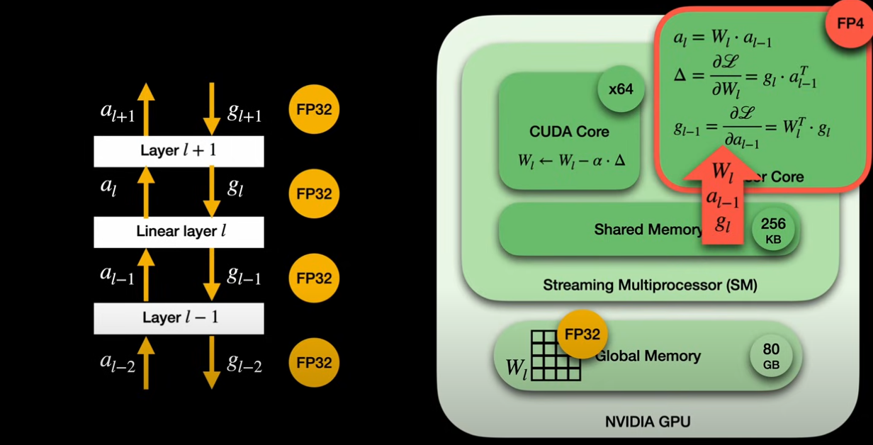
The streaming multiprocessor (SM) is the fundamental compute unit within an Nvidia GPU, containing CUDA cores (for general operations) and Tensor Cores (for high-throughput matrix multiplications). All cores share a faster on-chip shared memory.

Linear Layers and Matrix Multiplications: Linear layers, crucial to fully quantized training, involve matrix multiplications in both the forward pass (activations multiplied by weights) and the backward pass (gradient calculations from the chain rule). These three core matrix multiplications are executed by Tensor Cores.
Data Flow in FP4 Training
- Weights: The “master copy” of weights resides in global memory in full precision. A CUDA core reads this, quantizes it to FP4, and places it into the shared memory for Tensor Core access.
- Input Activations and Gradients: These flow through the network in high precision (FP32 or BF16) between layers. A CUDA core quantizes them to FP4 before they enter the Tensor Core.
- Outputs: Tensor Cores produce results in FP8. A CUDA core then upcasts these values to FP32 when applying model updates, matching the precision of the master weights.
Memory Efficiency: Bringing down inputs from FP32 to FP4 reduces memory pressure on Tensor Cores by eight times, which is critical as they are bottlenecked by memory.
Distinction from Quantization-Aware Training (QAT): While QAT, used by 1-bit LLMs, makes the forward pass “aware” of quantization, it still performs all Tensor Core multiplications in high precision (FP32). This means QAT does not lead to the same training efficiency gains as fully quantized training.

GGUF quantization

Refer GGUF (Generic Graph Universal Format)

Model Quantization

Table of Contents

Model Compression

Quantization

Example

Types

Legacy Quants (Oldest)

K-Quants (Smarter Blocks)

I-Quants (Vector Quantization)

Dequantize

Fixed-Point Arithmetic

Example:

One-Size Doesn’t Fit All

Types of Quantization Granularity

Per-Layer Quantization (Coarse-Grained)

Example:

Per-Channel (or Per-Row) Quantization (Fine-Grained)

Example:

Quantization Names Decoded

Pre traning Quantization

GGUF quantization

Resources

Graph View

Table of Contents