Convolutional neural network

A Convolutional Neural Network (CNN) is a type of neural network specifically designed to process grid-like data, most commonly images. Images are grids of pixels (height × width × channels), and CNNs are great at detecting patterns like edges, textures, shapes at various levels of complexity.

At a high level, a CNN does:

1. Feature extraction – Detects patterns in the image.
2. Feature combination – Combines simple features (like edges) into complex features (like shapes, objects).
3. Classification (or other tasks) – Uses extracted features to make predictions (e.g., this is a cat).

The key building blocks of CNNs are:

1. Convolutional layers – Apply filters/kernels to detect patterns.
2. Activation functions – Introduce non-linearity (ReLU is most common).
3. Pooling layers – Reduce spatial size while keeping important info.
4. Fully connected layers – Combine features for final prediction.

Convolution and Kernels

At its core, convolution is a mathematical operation that combines two functions to produce a third function. In the context of images:

• One function → the image (a grid of pixel values).
• Other function → the kernel/filter (small matrix used to detect patterns).
• Result → a new image highlighting certain features (edges, textures, etc.).

1. Place the kernel over a patch of the image.
2. Multiply each kernel value by the corresponding pixel value.
3. Sum the results → this gives a feature response.
4. Slide the kernel across the entire image → build a feature map.

So convolution is like scanning the image with a small “lens” that picks up certain patterns.

Mathematical Formula (2D convolution) For an image $I$ and kernel $K$:

$$S(i,j)=(I\ast K)(i,j)=\sum _m\sum _{n}I(i+m,j+n)\cdot K(m,n)$$

• $i,j$ → position in the output feature map.
• $m,n$ → indices in the kernel.
• The kernel slides across the image → each position gives one output.

A kernel (or filter) is a small matrix that slides over the image and performs convolution. Convolution is essentially a weighted sum of pixel values, highlighting certain features.

• Size: usually 3×3, 5×5, 7×7. Larger kernels capture bigger patterns.

• Learnable: In CNNs, kernels are not manually set. The network learns the best kernel values during training.
• Multiple kernels: A layer can have many kernels → each detects a different feature.

Types of Kernels

Kernels are the pattern detectors. Different kernels detect different features. Some common types:

** Edge detection kernels**

1. Vertical edge detection

$$K_v=\left[\begin{array}{ccc}-1& 0& 1\\ -1& 0& 1\\ -1& 0& 1\end{array}\right]$$

• Detects vertical edges.
• Left side dark, right side bright → high response.

2. Horizontal edge detection

$$K_h=\left[\begin{array}{ccc}-1& -1& -1\\ 0& 0& 0\\ 1& 1& 1\end{array}\right]$$

• Detects horizontal edges.
• Top dark, bottom bright → high response.

Sharpening kernel

$$K_s=\left[\begin{array}{ccc}0& -1& 0\\ -1& 5& -1\\ 0& -1& 0\end{array}\right]$$

• Emphasizes changes in intensity → makes image look sharper.

c) Blurring / Smoothing kernel

$$K_b=\frac{1}{9}\left[\begin{array}{ccc}1& 1& 1\\ 1& 1& 1\\ 1& 1& 1\end{array}\right]$$

• Averages nearby pixels → smooths the image / removes noise.

d) Emboss / Feature highlighting kernel

$$K_e=\left[\begin{array}{ccc}-2& -1& 0\\ -1& 1& 1\\ 0& 1& 2\end{array}\right]$$

• Highlights textures → makes parts of the image look 3D.

Example of vertical edge detection

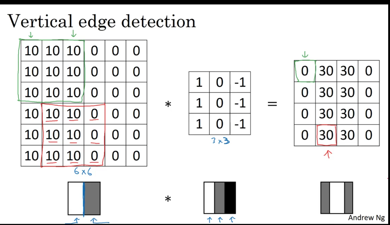
Left matrix (6×6 image patch)

10 10 10 0 0 0

10 10 10 0 0 0

10 10 10 0 0 0

10 10 10 0 0 0

10 10 10 0 0 0

10 10 10 0 0 0

• This represents a grayscale image where the pixel intensity ranges from 0 (black) to some higher number (white/bright).
• You can see a clear vertical edge between the left “bright” region (10) and right “dark” region (0). At a high level, a CNN does:

Feature extraction – Detects patterns in the image.

Feature combination – Combines simple features (like edges) into complex features (like shapes, objects).

Classification (or other tasks) – Uses extracted features to make predictions (e.g., this is a cat).

The key building blocks of CNNs are:

Convolutional layers – Apply filters/kernels to detect patterns.

Activation functions – Introduce non-linearity (ReLU is most common).

Pooling layers – Reduce spatial size while keeping important info.

Fully connected layers – Combine features for final prediction. Middle matrix (3×3 filter / kernel)

1 0 -1

1 0 -1

1 0 -1

• This is a vertical edge-detection kernel.
• The 1s detect bright pixels on the left, -1s detect dark pixels on the right, and 0s ignore the middle column.

Right matrix (output)

0 30 30 0

0 30 30 0

0 30 30 0

0 30 30 0

• This is the feature map (result of convolution).

• It highlights the vertical edges in the image. Values like 30 indicate strong vertical edges.

How Convolution Works Step by Step

Convolution slides the kernel over the image. For each position:

Step formula:

$$\text{output}[i,j]=\sum _{m,n}(\text{image}[i+m,j+n]\times \text{kernel}[m,n])$$

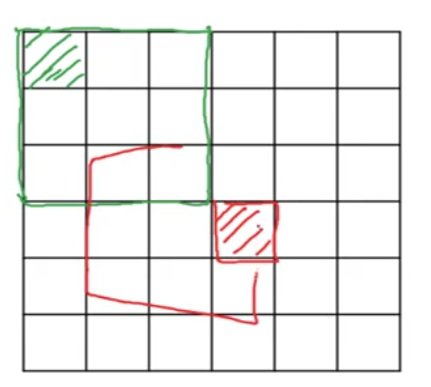
Example using the first 3×3 patch (green box):

Image patch: Kernel: Multiply & sum:

10 10 10 1 0 -1 10*1 + 10*0 + 10*-1 = 10 - 10 = 0

10 10 10 1 0 -1 10*1 + 10*0 + 10*-1 = 0

10 10 10 1 0 -1 10*1 + 10*0 + 10*-1 = 0

Sum = 0

• No edge detected here because the patch is uniform.

Next patch (red box):

10 10 0 1 0 -1 10*1 + 10*0 + 0*-1 = 10

10 10 0 1 0 -1 10

10 10 0 1 0 -1 10

Sum = 30

• Strong vertical edge detected → highlighted in output as 30.

Padding

Padding allows the convolution to cover all areas of the image, including the edges and corners, and can help in controlling the output dimensions. This image illustrates both the concept of padding and the resulting changes to the output size when padding is applied.

The convolution is performed on a 6x6 image. the filter (a 3x3) slides over the image, but if the filter is applied to the edges, it would leave out some areas of the image near the borders which is not covered effectively it only used once not used effectively Padding prevents this issue.

• Without padding, applying a 3x3 filter to a 6x6 image results in an output of 4x4
• This is calculated by the formula:

$$\text{Output size}=\left(\frac{n-f+1}{\text{stride}}\right)$$

where:

• $n$ is the input size (6 in this case).
• $f$ is the filter size (3 here).
• The stride is typically 1 unless otherwise specified.

Thus, the formula for this example gives $(6-3+1)=4$ for both dimensions, resulting in a 4x4 output.

Types of Padding:

There are generally two types of padding:

• Valid padding: No padding is added to the input, and the output size decreases after convolution (as seen with the 4x4 output).

• Same padding: Padding is added to ensure that the output size is the same as the input size. For example, if the input is 6x6 and you use a 3x3 filter with same padding, you’d get a 6x6 output.

Strided Convolution in CNNs

Strided Convolution is a technique used in Convolutional Neural Networks (CNNs) where the filter (or kernel) moves across the input image with a step size greater than 1. The step size is known as the stride. This concept is important because it allows for reducing the spatial dimensions (height and width) of the feature map.

In a regular convolution (stride = 1), the filter moves pixel by pixel across the image, producing an output at every position where it fully overlaps with the input image.

Strided convolution reduces the size of the output feature map. The output size for a convolution operation with stride $S$ can be calculated using the formula:

$$\text{Output size}=\left(\frac{n-f}{S}+1\right)$$

• $n$ is the input size (height or width of the input image).
• $f$ is the filter size (height or width of the filter).
• $S$ is the stride (step size).

Pooling layers

Max pooling

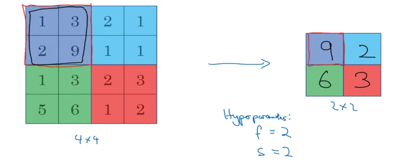
In max pooling, the algorithm selects the maximum value from a subset of the image defined by a filter (also called a pool) and moves it over the image to reduce its size. It retains only the most significant features, making the representation more abstract.

Average pooling Take average of the area

Forward and backpropgation

Imagine we have a very simple CNN with:

• Input array $[2,3]$
• Filter (kernel) $[1,1]$
• True Label: 6 (We want our CNN to predict this value)
• Loss function: Squared Error (how far the predicted value is from the true label)

Now, let’s go through this step by step.

Step 1: Forward Pass (Convolution)

1. Perform the convolution:

The filter is applied to the input with a stride of 1, so the output of the convolution is calculated as:

$$\text{Output}=(2\times 1)+(3\times 1)=2+3=5$$

The predicted output is 5.

2. Calculate the loss:

The loss (error) is calculated as the difference between the predicted output (5) and the true label (6):

$$\text{Loss}=(5-6{)}^2=1$$

So, the loss is 1. Now we want to reduce this loss by adjusting the filter values during the backpropagation step.

Step 2: Backpropagation to Find Gradients

Backpropagation allows us to calculate how much the filters contributed to the loss, and we want to adjust them accordingly.

To adjust the filters, we need to calculate the gradient of the loss with respect to each filter weight. This means we need to find how much the filter weights $w_1$ and $w_2$ (the two weights in the filter) need to change to reduce the loss.

The Chain Rule

We will use the chain rule of calculus to calculate how the loss depends on each filter weight. The key idea is that we break down the calculation into smaller parts.

1. Calculate the gradient of the loss with respect to the output:

The output of the convolution is $5$. We need to calculate how much the loss changes with respect to this output:

$$\frac{\partial \text{Loss}}{\partial \text{Output}}=2\times (\text{Output}-\text{True Value})=2\times (5-6)=-2$$

This tells us that the output needs to be decreased to reduce the loss.

2. Calculate the gradient of the output with respect to the filter weights:

Now, we calculate how the output depends on the filter weights:

• The first filter weight $w_1$ is multiplied by the first input value $2$, so:

$$\frac{\partial \text{Output}}{\partial w_1}=2$$

• The second filter weight $w_2$ is multiplied by the second input value $3$, so:

$$\frac{\partial \text{Output}}{\partial w_2}=3$$

3. Apply the chain rule to get the gradient of the loss with respect to the filter weights:

Using the chain rule, we multiply the gradient from Step 1 (the loss with respect to the output) by the gradients from Step 2 (the output with respect to the filter weights):

• For the first filter weight:

$$\frac{\partial \text{Loss}}{\partial w_1}=\frac{\partial \text{Loss}}{\partial \text{Output}}\times \frac{\partial \text{Output}}{\partial w_1}=-2\times 2=-4$$

• For the second filter weight:

$$\frac{\partial \text{Loss}}{\partial w_2}=\frac{\partial \text{Loss}}{\partial \text{Output}}\times \frac{\partial \text{Output}}{\partial w_2}=-2\times 3=-6$$

Step 3: Update the Filter Weights Using Gradient Descent

Now that we have the gradients, we can use gradient descent to update the filter weights.

Let’s assume the learning rate $\eta =0.1$.

We update each filter weight using the gradient descent rule:

$w_{\text{new}}=w_{\text{old}}-\eta \times \frac{\partial \text{Loss}}{\partial w}$

For the first filter weight: $w_1^{\text{new}}=w_1^{\text{old}}-0.1\times (-4)=1-(-0.4)=1+0.4=1.4$

For the second filter weight: $w_2^{\text{new}}=w_2^{\text{old}}-0.1\times (-6)=1-(-0.6)=1+0.6=1.6$

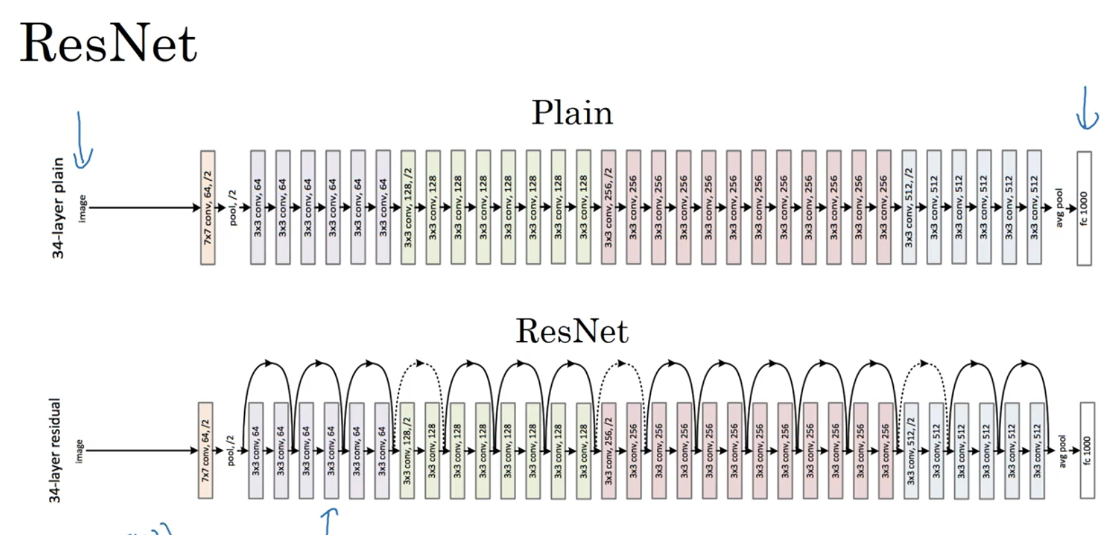
Residual Block

In traditional deep neural networks, as the number of layers increases, it becomes difficult to train the network due to issues like vanishing gradients. Residual blocks address this problem by adding a shortcut connection (also called a skip connection) that directly passes the input from an earlier layer to a deeper layer.

This shortcut allows the model to learn the difference between the input and the output, making it easier to learn identity mappings and improve training. Instead of learning the mapping y=f(x)y = f(x)y=f(x), a residual block learns y=f(x)+xy = f(x) + xy=f(x)+x, where x is the input and f(x)f(x)f(x) is the transformation.

Let say we have a 34-layer network, and you’re adding residual connections (or shortcuts) that allow the network to skip intermediate layers when performing backpropagation. But in the forward pass, all 34 layers are still used to process the input and make predictions.

Tools

• An interactive node-link visualization of convolutional neural networks,

Resources

• https://adeshpande3.github.io/A-Beginner%27s-Guide-To-Understanding-Convolutional-Neural-Networks/