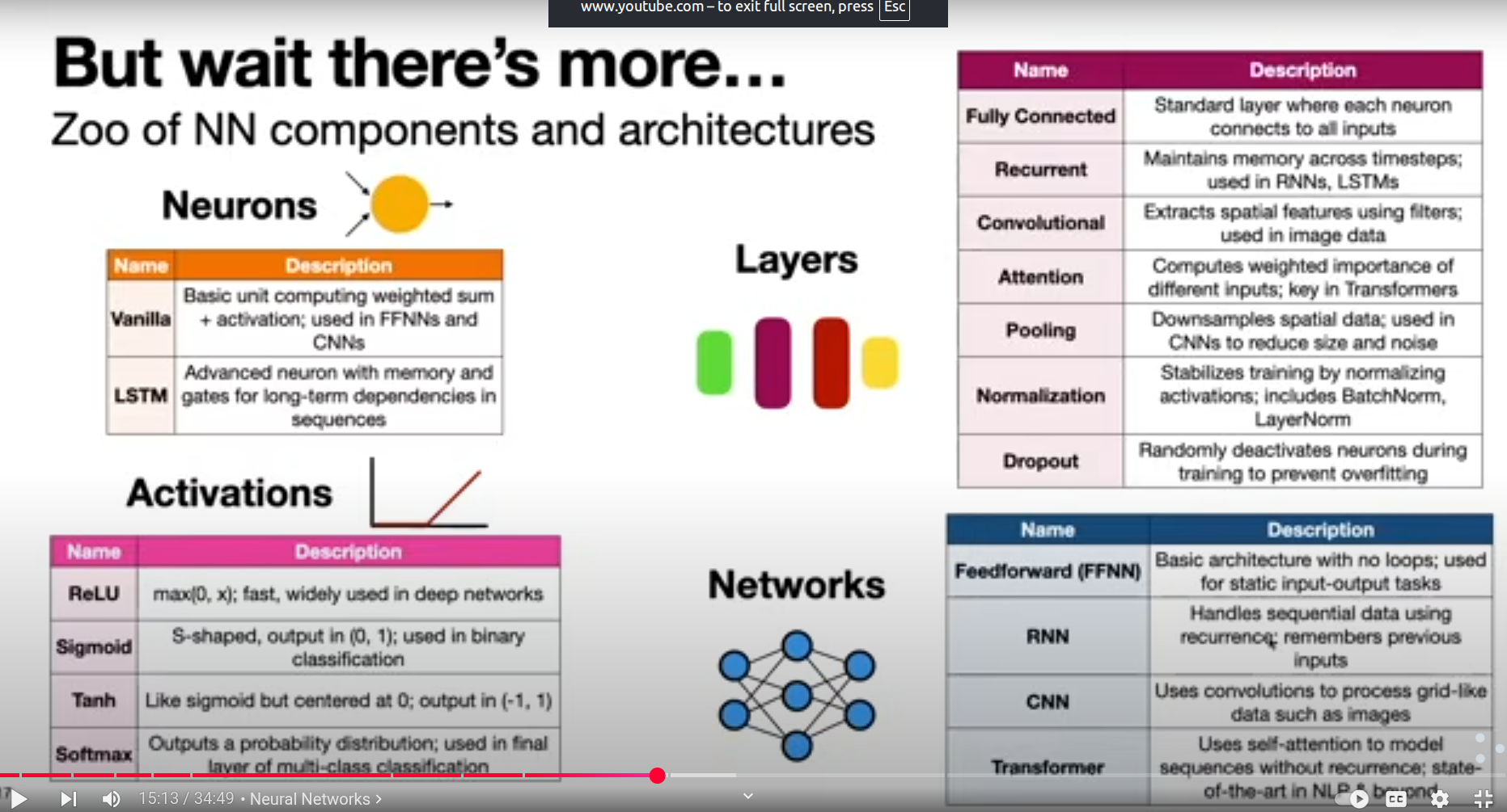
Perceptron
bias →The addition of bias reduces the variance and hence introduces flexibility and better generalisation to the neural network.
Activation Function
- Linear
- Sigmoid or Logistic Activation Function
- Tanh or hyperbolic tangent Activation Function
- ReLU (Rectified Linear Unit) Activation Function ( most used activation function in the world right now)
NOTE: neural nets don’t directly learn curved spirals they learn to transform the input space until straight lines are enough.
Multiple input Preceptron formula
. Simple Line (2D) Equation of a line:
- = slope,
- = intercept.
This is basically 1 input variable () and two parameters ().
Generalizing to Many Inputs
When we move to multiple inputs ():
- Each input has its own weight .
- is the bias (like intercept ).
Writing in Matrix Form
Instead of writing long sums, we use vectors & dot products.
-
Inputs:
-
Weights:
-
Dot product:
So:
Activation Function
The perceptron then applies a non-linearity (sigmoid, ReLU, etc.):
A matrix representation
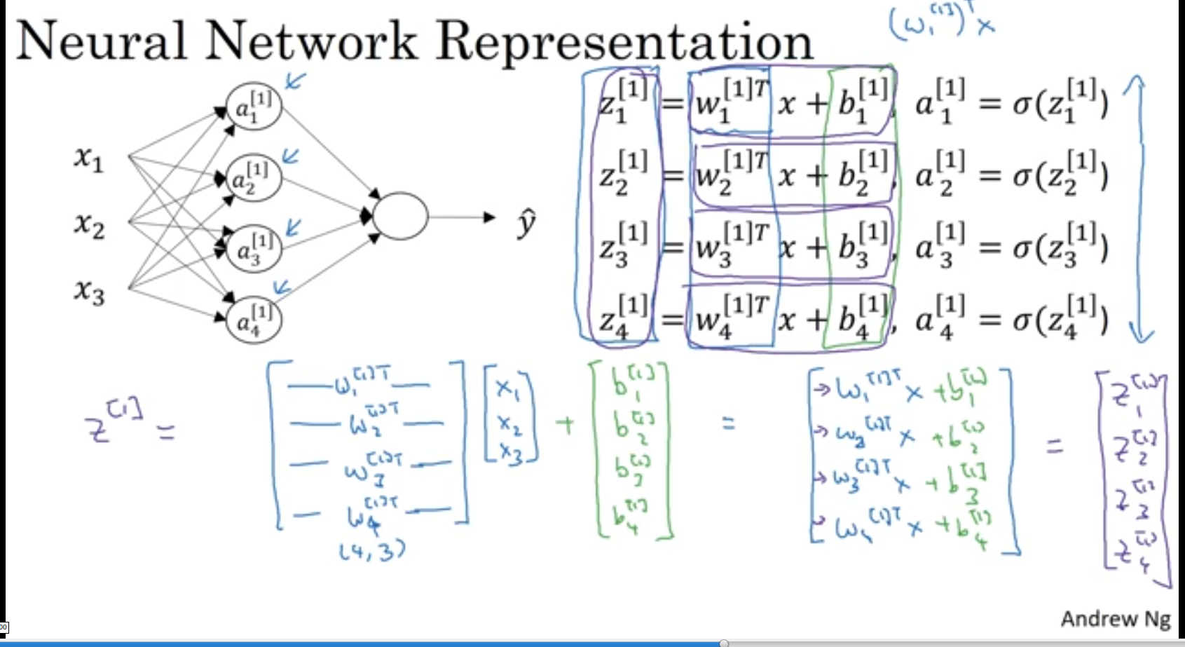
Every layer in a neural network follows this rule:
- : weights for layer
- : biases for layer
- : activations from the previous layer
- : activations for this layer (after activation function)
- : activation function (sigmoid, ReLU, etc.)
Linear step (z) + Nonlinear step (σ)
we have:
- Inputs:
- Hidden layer (layer 1): 4 neurons
- Output layer (layer 2): 1 neuron
Hidden Layer (Layer 1)
Input is . Formula:
- : size → 4 neurons, each sees 3 inputs
- : size → 3 inputs
- : size
- Result : size
- Apply activation:
Output Layer (Layer 2)
Input is the hidden layer output .
- : size → 1 output neuron, takes 4 inputs
- : size
- : size
- Result : size
- Apply activation:
This final value is our prediction .
Input (3,1) → Hidden layer (4,1) → Output (1,1)
Full matrix look Input:
Weights:
Bias:
Multiply:
That gives:
NEURONS--MATRIX-REPRESENTATION
- For each input we have different weight in the neurons we can represet the whole layer in single matrix like above z
- After activation: a^[1] = σ(z^[1]) → (4,1)
Note currently we only have single input like x1,x2 ,x3 let say we have 500 feature like 3* 500 we can just convert to matrix and do the parallel computaion
Weight intilization
The goal of weight initialization is to keep signals from shrinking or exploding as they pass through layers.
If values shrink → vanishing gradient If values explode → exploding gradient
| Method | Why it works | Best for |
|---|---|---|
| Random Init | Breaks symmetry but doesn’t control growth/shrink | Not recommended except for small models |
| Xavier | Sigmoid/tanh compress signals → need balanced weights | Sigmoid, Tanh |
| He | ReLU kills half activations → needs stronger weights | ReLU, Leaky ReLU |
| LeCun | SELU self-normalizes → needs smaller weights | SELU |
| Orthogonal | RNN needs stable repeated multiplication | RNNs |
Normalization layers (BatchNorm / LayerNorm)
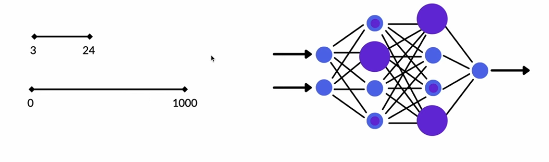
Layer normalization is a technique in deep learning that normalizes the inputs to a layer by computing the mean and standard deviation across all neurons for a single data point. This process stabilizes the training of neural networks, reduces internal covariate shift, and improves convergence by ensuring that the activation values have a consistent distribution.
If we did not do the and we have samll input and big input which make our weights to huge on some parts which is bad.
Normalization forces:
- Mean ≈ 0
- Variance ≈ 1
Which keeps activations from drifting into saturated regions of sigmoid/tanh and keeps ReLU inputs from going too large.
As a result:
- Derivatives for sigmoid/tanh stay in a region where they are not tiny.
- Intermediate activations don’t blow up → Jacobians don’t accumulate large values.
Normalization controls the distribution, stabilizing the product of derivatives.
we do on input data also check
Norimalization formual
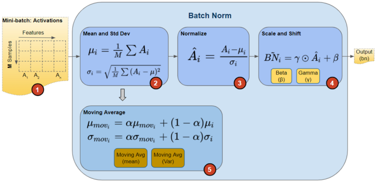
Batch Norm
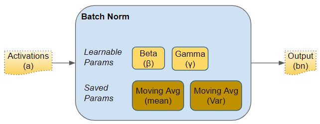
Batch Norm is just another network layer that gets inserted between a hidden layer and the next hidden layer. Its job is to take the outputs from the first hidden layer and normalize them before passing them on as the input of the next hidden layer.
Batch Norm vs layer norm
         feature1   feature2   feature3
sample1:    1          2          3
sample2:    4          5          6
sample3:    7          8          9
sample4:    1          3          5

BN uses ↓      BN uses ↓       BN uses ↓
   [1,4,7,1]     [2,5,8,3]       [3,6,9,5]


sample1 → [1,2,3]
sample2 → [4,5,6]
sample3 → [7,8,9]
sample4 → [1,3,5]

LN uses → only that row
BatchNorm
- Looks across ALL samples
- Normalizes per feature
- Needs big batch
- Behavior depends on mixing examples
LayerNorm
- Looks inside ONE sample only
- Normalizes per sample
- Works with batch size 1
- Used in Transformers, RNNs
BatchNorm compares each feature to the same feature in other samples.
LayerNorm compares each sample to itself.
Residual connection
A residual connection, or skip connection, is an architectural innovation in neural networks that bypasses one or more layers to feed the output of an earlier layer directly to a later layer. The core purpose is to enable the training of very deep networks by mitigating problems like vanishing gradients and performance degradation
Resources
- Batch Normalization: Accelerating Deep Network Training b y Reducing Internal Covariate Shift
- Batch Norm Explained Visually – How it works, and why neural networks need it
Regularization
Regularization = controls model flexibility so it learns stable, simple, general rules instead of memorizing.
If we dont do the regularization the model will only good at test and train data it will started memorize the data so to avoid we use regularization
Common methods:
- Weight decay (L2)
- L1 regularization
- Dropout
- Early stopping
- Data augmentation
- Batch norm
- Smaller models
- Noise injection
- Label smoothing
check machine learning regulaarization Here
Dropout
To prevent overfitting It works by randomly “dropping out” or deactivating a fraction of the neurons during each training step. This prevents the network from becoming too reliant on specific neurons and forces it to learn more robust features that generalize better to new data.
How Dropout Works:
- During Training: For each training step, each neuron in the network has a probability p of being dropped out (set to zero). This means the neuron doesn’t contribute to the forward pass or the backward pass (no weight update).
- For example, if the dropout rate is 0.5, there’s a 50% chance that each neuron will be deactivated in each forward pass.
- During Testing/Inference: Dropout is turned off during the testing phase. All neurons are active, but their weights are scaled down by a factor of 1−p1 - p1−p (i.e., 50% if p=0.5p = 0.5p=0.5) to ensure that the network does not become too confident about specific features.
Why Use Dropout?
- Prevent Overfitting: Dropout prevents the model from becoming too dependent on any single neuron. Without dropout, some neurons may “memorize” the training data, leading to overfitting. Dropout forces the network to learn redundant representations, making it more robust.
- Improves Generalization: By randomly removing neurons during training, dropout encourages the model to learn more generalized features, improving performance on unseen data.
Example: Imagine we are training a neural network with 4 neurons in a hidden layer, and we apply dropout with a rate of 0.5.
- During training, on each training step, there’s a 50% chance that each neuron will be dropped. So, we might end up with a configuration like this:
- Step 1: Neurons 1 and 4 are dropped, and the model trains with Neurons 2 and 3.
- Step 2: Neurons 2 and 3 are dropped, and the model trains with Neurons 1 and 4.
This prevents the network from relying too much on specific neurons and encourages it to generalize better.
Gradient Clipping
Gradient clipping is a technique used to prevent the exploding gradients problem during neural network training by scaling down gradients that exceed a certain threshold. This keeps the weight updates from becoming excessively large, which can cause the model to diverge and the training process to become unstable.
Gradient clipping is implemented in two variants:
- Clipping-by-value
- Clipping-by-norm
The idea behind clipping-by-value is simple. We define a minimum and a maximum clip value.
If a gradient exceeds some threshold value, we clip that gradient to the threshold. If the gradient is less than the lower limit, then we clip that too, to the lower limit of the threshold.
The idea behind clipping-by-norm is similar to clipping-by-value. The difference is that we clip the gradients by multiplying the unit vector of the gradients with the threshold.
Exponentially Weighted Average (EWA)
The temperature walk-through is in Exponentially Weighted Average (EWA).
Resources
- https://towardsdatascience.com/what-is-a-perceptron-basics-of-neural-networks-c4cfea20c590
- https://medium.com/fintechexplained/neural-networks-bias-and-weights-10b53e6285da
- https://medium.com/the-theory-of-everything/understanding-activation-functions-in-neural-networks-9491262884e0
- https://towardsdatascience.com/activation-functions-neural-networks-1cbd9f8d91d6
- Deep Learning Interviews is home to hundreds of fully-solved problems, from a wide range of key topics in AI. It is designed to both rehearse interview or exam-specific topics and provide machine learning M.Sc./Ph.D. https://arxiv.org/pdf/2201.00650
- https://deeplearning.neuromatch.io/tutorials/W1D1_BasicsAndPytorch/chapter_title.html
Understanding AI - Lesson 1 / 15: A Simple Neural Network from scrach
Maths