Generative modeling is a branch of machine learning that involves training a model to produce new data that is similar to a given dataset.

The Generative Modeling Framework

We have a dataset of observations
We assume that the observations have been generated according to some unknown distribution, P(data).
We want to build a generative model P(model) that mimics P(data). If we achieve thisgoal, we can sample from pmodel to generate observations that appear to have been drawn from pdata.

Discriminative Models

These learn: P(Y|X) = “Given input X, what’s the probability of output Y?”

Example: Looking at a photo (X) → Is it a cat or dog? (Y)

Logistic regression
Most neural networks you’ve seen

What they do: Draw boundaries between classes

Generative Models

These learn: P(X, Y) = “What’s the joint probability of both X and Y occurring together?”

The key difference: Generative models learn how the data itself is distributed.

Why this matters: If you know the distribution of data, you can generate new data from that distribution!

Example:

Discriminative: “Is this face male or female?”
Generative: “Generate a new realistic face”

This are accept input in one format and produce the ouutput in different format

Text to image
Text to audio

Deep Generative Models

Traditional generative models (like Gaussian Mixture Models, Hidden Markov Models) work for simple data.

But for high-dimensional, complex data like images, audio, or text they fail.

Deep learning provides powerful nonlinear functions (via neural nets), so we can model very complex data distributions.

Deep Generative Models assume:

Data $x$ is generated from some hidden variables (latent space) $z$ .
Neural networks learn the mapping between latent variables ↔ data.

z \sim p (z) \to x \sim p (x ∣ z)

Example:

$z$ = a compressed “concept” of a face (gender, hair, smile).
$x$ = the actual pixels of the face.

Types of Deep Generative Models

Latent variable Models Variational Autoencoders (VAEs) Learn to compress input → latent space → reconstruct input. Latent space has structure, so we can sample new points to generate new data. Example: generate new handwritten digits after training on MNIST. Generative Adversarial Networks (GANs) Two networks: Generator*: tries to create fake but realistic data. Discriminator: tries to distinguish real vs fake. They play a game until generator produces very realistic samples. Example: Deepfake images.

Autoregressive Models

Model data as a sequence, predict next element step by step.
Example: PixelRNN, GPT (for text).

Diffusion Models (modern SOTA)

Learn to gradually remove noise from data → generate high-quality samples.
Example: Stable Diffusion, DALL·E.

Autoencoders

An autoencoder is simply a neural network that is trained to perform the task of encoding and decoding an item, such that the output from this process is as close to the original item as possible

An autoencoder is a neural network made up of two parts:

An encoder network that compresses high-dimensional input data such as an image into a lower-dimensional embedding vector
A decoder network that decompresses a given embedding vector back to the original domain (e.g., back to an image)

The embedding (z) is a compression of the original image into a lower dimensional latent space. The idea is that by choosing any point in the latent space, we can generate novel images by passing this point through the decoder, since the decoder has learned how to convert points in the latent space into viable images.

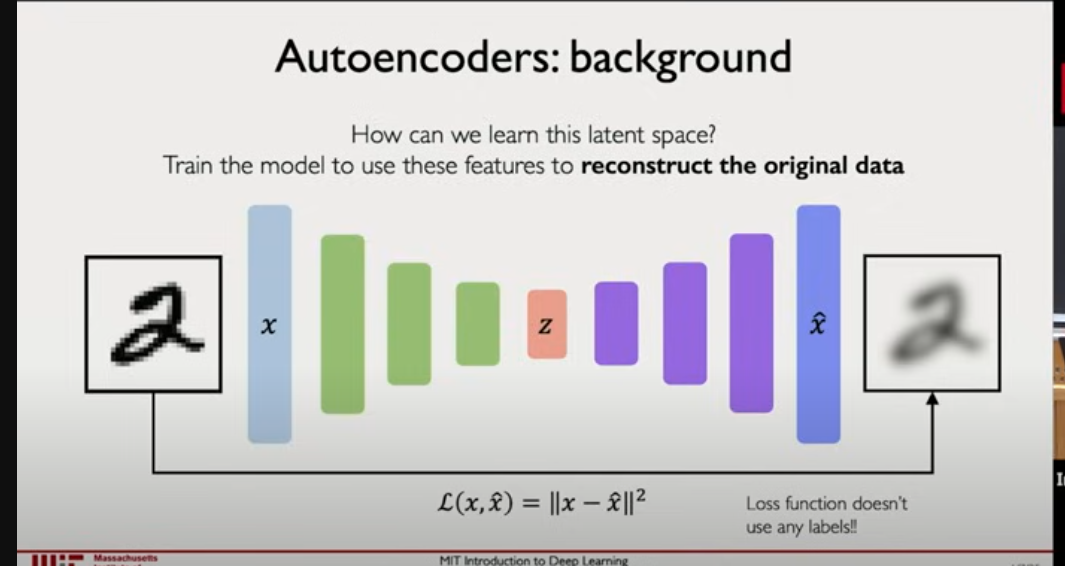
What it do was convert the data in to latent space (in low dimension ) using encoder and again use decoder to reconstruct the same data using decoder and now the compare the loss and adjust it like unsuppervised learning where it learn automatically no labled data in needed

Input (x): The original image (e.g., digit “2” from MNIST).
Encoder (left side, green bars): Neural network that compresses input into a small representation.
Latent Variable (z): The compressed code, the “essence” of the image.
Decoder (right side, purple bars): Neural network that expands the latent variable back to the image.
**Reconstructed Output : The reconstructed digit, ideally similar to the input.

Variational Autoencoders (VAEs)

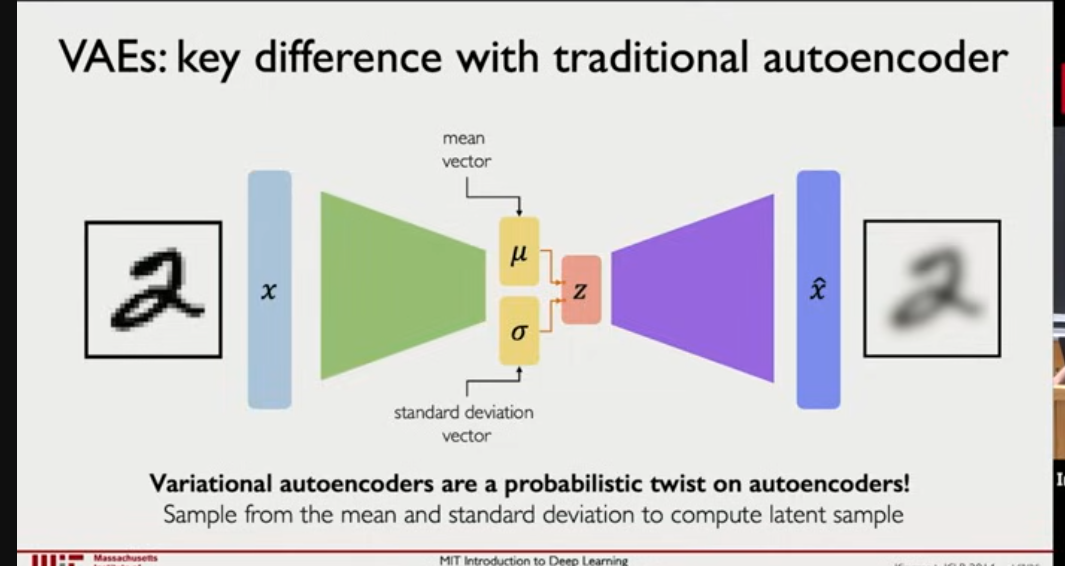
Input Image (x): For example, a handwritten digit (like a 2 from MNIST).
Encoder Network: Instead of encoding directly to a point in latent space, the encoder outputs:
- A mean vector (μ)
- A standard deviation vector (σ)

What “mean” and “std” mean in plain terms

Suppose these are exam marks:

Marks = [35, 38, 40, 72, 75, 78]

Mean (average)

Add everything and divide:

mean = (35+38+40+72+75+78) / 6 ≈ 56

Meaning:

Mean tells you the center of the group.

So:

Below 56 → below average
Above 56 → above average

Standard deviation (std)

Std answers a different question:

“On average, how far are students from the mean?”

Here, roughly:

std ≈ 18

So:

Most students are about 18 marks away from the average.

What “mean 0, std 1” means (this is crucial)

Now we change the scale.

Instead of marks, we measure distance from average, in units of spread.

z = (mark - mean) / std

This does TWO things:

Subtract mean → center becomes 0
Divide by std → spread becomes 1

Concrete examples

Mark	Calculation	z-score
56	(56−56)/18	0
74	(74−56)/18	+1
38	(38−56)/18	−1
92	(92−56)/18	+2

So now:

z = 0 → average student
z = +1 → 1 standard deviation above average
z = −1 → 1 standard deviation below average

So the Z variable will be make the input around mean and STD

Latent Sampling (z):
- A sample z is drawn from the distribution N(μ, σ²).
- This is the key probabilistic twist!
- The sampling is done using the reparameterization trick:

z = μ + σ * ε, where ε ~ N(0, I)

Decoder Network: Decodes the sample z back into a reconstruction x̂ (the blurred image).

“Variational autoencoders are a probabilistic twist on autoencoders!”

“Sample from the mean and standard deviation to compute latent sample.”

The probabilistic nature allows for:
Smooth interpolation in latent space
Generative modeling (e.g., creating new digits)
Regularization via KL divergence

So basically we going to find the probablity distribution of our input data and map that to latent space

kullback leibler divergence

Let’s name them:

P(x) → true / actual data distribution
Q(x) → model predicted distribution

Why simple subtraction fails (your intuition is correct)

First idea (natural but wrong):

P(x) - Q(x)

Why this fails:

Positive and negative cancel out
- Overestimate in one region
- Underestimate in another
- Total difference can look small even when distributions are very different
Scale problem
- Probabilities are relative, not absolute
- A difference of 0.1 means very different things depending on context
No directional meaning
- It doesn’t tell how wrong you are
- Just “different”, but not in what way

So subtraction loses structure and meaning.

Your note:

“if we subtract we miss lot of thing”

This is exactly right.

Why ratios are more informative than differences

Next idea (this is the key insight):

Instead of subtracting, compare them by division

So we look at:

P(x) / Q(x)

Why this is powerful:

If P(x) / Q(x) = 1 → perfect match
If > 1 → model underestimated this event
If < 1 → model overestimated this event

This ratio answers:

“How many times more (or less) likely is reality compared to my model?”

This is scale-free, directional, and meaningful.

Your note:

“if we divide predicted and actual we get the ratio which tell how much we are from actual data if the ratio is less then 1 or greater then 1”

Correct this is the fundamental idea behind KL divergence.

Why we take the logarithm of the ratio

Now we have a ratio:

P(x) / Q(x)

But raw ratios have problems:

Very large numbers
Hard to aggregate
Multiplicative errors stack badly

So we apply log:

log(P(x) / Q(x))

Why log?

Turns multiplication into addition
- Easier to sum across events
Symmetric interpretation
- Overestimating and underestimating are treated consistently
Information meaning
- This log ratio literally measures surprise
- How much information is lost when using Q instead of P

This comes directly from information theory, not ML tricks.

Why we weight by the true distribution P(x)

Now we have:

log(P(x) / Q(x))

But this measures error at a single point x.

We need a global measure over all possible x.

So we take an expectation:

Σ P(x) * log(P(x) / Q(x))

Why weight by P(x)?

Because:

Errors where data actually occurs matter more
Errors in rare/impossible regions don’t matter much

This means:

We are measuring the average extra surprise caused by using Q when the world actually follows P.

This is the final form of KL divergence.

Final KL divergence (what we “invented”)

After all this reasoning, we arrive at:

KL(P || Q) = Σ P(x) log(P(x) / Q(x))

What KL divergence is really measuring (mental model)

Think of it this way:

P = how the world truly generates data
Q = how your model thinks data is generated

KL divergence measures:

“How much extra information (or coding cost or surprise) do I incur by believing Q when reality is actually P?”

Lower KL → model distribution closer to reality Zero KL → perfect match

Why KL is used in encoders (VAEs, etc.)

In encoders:

The encoder outputs a probability distribution (not a single value)
We want this distribution to be close to a target distribution
So we use KL divergence as the loss

My understanding

We have complex data (images, text, audio) with thousands of dimensions, but the real factors that create this data are much simpler (like 10-20 things). We want to discover these hidden factors.

Example: A face photo has 1 million pixels, but is created by:

Age (young/old)
Gender (male/female)
Smile (yes/no)
Lighting (bright/dark)
Hair style, etc.

VAE tries to discover these factors automatically.

What the Encoder Actually Does:

It’s like a descriptive artist looking at an image and saying:
“I see a face. Let me describe it using my learned vocabulary…”

The Vocabulary is (μ, σ):

μ: “This is what I see most clearly”
σ: “This is how sure I am about what I see”

Example for digit “7”:

Artist sees a “7” and thinks: “Shape: Definitely like a ‘7’ (μ₁=0.8, σ₁=0.1) ← Very sure Tilt: Maybe slightly right-leaning (μ₂=0.3, σ₂=0.4) ← Less sure”

The neural network learns that:

All “7”s should have similar descriptions
Clear features get small σ (high confidence)
Ambiguous features get larger σ (less confidence)

THE REPARAMETERIZATION TRICK: CONTROLLED RANDOMNESS

The Problem in Simple Terms:

If we just say “pick a random z from this distribution”, we can’t learn from it because randomness has no gradient.

Also it will produce the same z value for same input to avoid we add randomness and make the probablity distribution

z = μ + σ × ε

Think of it like baking:

ε: Basic ingredients (flour, sugar) - always the same types
μ: Recipe adjustments (“add 200g of flour”) - learnable
σ: How precise the recipe is (“±10g”) - learnable

Why This Works:

The randomness (ε) is fixed and separate
We learn how to INTERPRET this randomness via μ and σ
Gradients can flow through μ and σ

For “7” image: μ = 0.5 (center point for “7-ness”) σ = 0.2 (how much “7-ness” can vary) ε = 0.3 (random number from standard jar)

z = 0.5 + 0.2 × 0.3 = 0.56

This z represents: “A fairly typical 7, maybe a bit more 7-ish than average”

KL DIVERGENCE: THE RULE ENFORCER

The KL Divergence term specifically pushes the encoder’s outputs to match the standard normal distribution N(0, 1).

A teacher that says: “Use the standard measurement system!”

Without KL (Chaos):

Different images describe themselves in different units:

Image 1: “My 7-ness is 283.5 units”
Image 2: “My 7-ness is -147.2 units”
Image 3: “My 7-ness is 0.0004 units”

No consistency! Can’t compare or interpolate.

With KL (Order):

KL says: “Everyone use the standard scale of -3 to +3!”

Now all “7”s describe themselves between 0.2 and 0.8
All “1”s between -0.9 and -0.5
All “0”s between 0.7 and 1.2

The Penalty System:

KL looks at your (μ, σ) and says:

If you’re too extreme:

Network: “This is a very special 7! μ=5.0, σ=0.001” KL: “Whoa! Too far from (0,1)! Penalty: 12.3 points” → Network learns to be less extreme

If you’re reasonable:

Network: “This is a typical 7: μ=0.3, σ=0.8”
KL: “Good! Close to standard. Penalty: 0.2 points” → Network keeps doing this

What KL Actually Measures:

“How surprised would I be if I expected a standard normal distribution but got your distribution instead?”

WHY N(0,1)? THE UNIVERSAL LANGUAGE

Analogy: Time Zones

New York: EST (UTC-5)
London: GMT (UTC+0)
Tokyo: JST (UTC+9)

To compare times, we convert to UTC. Similarly:

To compare latent codes, we convert to N(0,1)

Benefits of This “Universal Language”:

Comparable: Can compare any two images
Interpolatable: Can blend between images
Samplable: Can create new images by sampling

Here is the correct mental model, step by step:

Input x
Encoder produces using neural network we try to find the 2 feature from the input (μ, σ) (so the neural network try find pattern )
We add controlled noise to create z such that we dont get always same output for same input

z = μ + σ · ε

So we use KL Divergence loss function to find how the (μ, σ) are with our distribution and we adjust thar such that we able to get the normal distrubution for our data

The formula for normal distribution is ε ∼ N(0,1) the mean will be 0 and standard devation will be 1 we make sure our predicted (μ, σ) also align with this such our Z will be a probablity distribution

Decoder reconstructs x̂ from z
Loss has two independent parts:
- Reconstruction loss → “did we rebuild x?”
- KL penalty → “did μ and σ obey the rule?”

Nothing is “mapped to a distribution”.

So we try to create a normal distribution from the input data

z = μ + σ · ε

μ and σ are neural networks learn from input data the ε for randomness

import torch
import torch.nn as nn
import torch.nn.functional as F
 
class VAE(nn.Module):
    def __init__(self, input_dim=784, hidden_dim=400, latent_dim=20):
        super(VAE, self).__init__()
 
        # --- Encoder ---
        self.fc1 = nn.Linear(input_dim, hidden_dim)
        self.fc_mu = nn.Linear(hidden_dim, latent_dim)    # Mean
        self.fc_logvar = nn.Linear(hidden_dim, latent_dim) # Log Variance
 
        # --- Decoder ---
        self.fc3 = nn.Linear(latent_dim, hidden_dim)
        self.fc4 = nn.Linear(hidden_dim, input_dim)
 
    def encode(self, x):
        h = F.relu(self.fc1(x))
        return self.fc_mu(h), self.fc_logvar(h)
 
    def reparameterize(self, mu, logvar):
        # Reparameterization trick: z = mu + std * epsilon
        std = torch.exp(0.5 * logvar)
        eps = torch.randn_like(std)
        return mu + eps * std
 
    def decode(self, z):
        h = F.relu(self.fc3(z))
        return torch.sigmoid(self.fc4(h)) # Sigmoid for pixel values [0, 1]
 
    def forward(self, x):
        x = x.view(-1, 784) # Flatten
        mu, logvar = self.encode(x)
        z = self.reparameterize(mu, logvar)
        return self.decode(z), mu, logvar
 
# --- Loss Function ---
def loss_function(recon_x, x, mu, logvar):
    # 1. Reconstruction Loss (Binary Cross Entropy is standard for MNIST)
    BCE = F.binary_cross_entropy(recon_x, x.view(-1, 784), reduction='sum')
 
    # 2. KL Divergence: measure how much the latent variables deviate from a normal distribution
    # Equation: 0.5 * sum(1 + log(sigma^2) - mu^2 - sigma^2)
    KLD = -0.5 * torch.sum(1 + logvar - mu.pow(2) - logvar.exp())
 
    return BCE + KLD

To understand how a VAE works, let’s trace a single 28x28 pixel image (like a digit “7” from the MNIST dataset) as it moves through the network.

1. The Input Layer

Input: A grayscale image of size .
Transformation: We flatten this image into a single vector of 784 values (since ).
Data State: A tensor of shape [1, 784] (assuming batch size 1).

2. The Encoder (Dimensionality Reduction)

The encoder’s job is to compress the 784 pixels into a much smaller set of numbers that represent “features” (like the tilt of the “7” or the thickness of the lines).

Hidden Layer: The 784 values pass through a Linear layer (with ReLU) to become 400 values.
Bottleneck: These 400 values are then split into two separate paths:

Mu (): A vector representing the “mean” (e.g., 20 values).
Log-Variance (): A vector representing the “uncertainty” or spread (20 values).

Data State: We now have two vectors of shape [1, 20].

3. The Reparameterization Trick (The Magic Step)

We can’t just pick the mean (); we need to sample from a distribution to keep the model “creative.”

We take a random noise sample (epsilon) from a Standard Normal Distribution ( to ).
We calculate the actual sample using:

Data State: A single “Latent Vector” of shape [1, 20]. This is the compressed “essence” of your image.

4. The Decoder (Reconstruction)

Now we try to turn those 20 numbers back into a full image.

Upscaling: The 20 values pass through a Linear layer to become 400 values again.
Output Layer: Those 400 values pass through a final Linear layer to become 784 values.
Activation: We use a Sigmoid function to ensure every value is between and (just like pixel intensities).
Data State: A tensor of shape [1, 784].

5. The Output & Loss

Output: We “unflatten” the 784 values back into a grid. It should look like a slightly blurry version of the original “7”.
The Comparison:
Reconstruction Loss: Compares the output pixels to the input pixels. If they don’t match, the model adjusts.
KL Divergence: A “penalty” that forces the Encoder to keep near and near . This ensures the latent space stays organized and doesn’t just “memorize” the input.

Summary Table: Data Transformation

Component	Input Shape	Output Shape	Purpose
Input	`(28, 28)`	`(784,)`	Flattening for the neural net.
Encoder	`(784,)`	`(20,)` (mu & var)	Compress pixels into “concepts”.
Latent Space ()	`(20,)`	`(20,)`	Add randomness (sampling).
Decoder	`(20,)`	`(784,)`	Rebuild image from concepts.
Output	`(784,)`	`(28, 28)`	Reshape back to image format.

Backpropgation This is called the Evidence Lower Bound (ELBO). It is a balance between two competing goals:

A. Reconstruction Loss (The “Realism” Term)

What it does: It measures how well the decoder rebuilt the image.
The Math: Usually Mean Squared Error (MSE) or Binary Cross Entropy (BCE).
Intuition: If the input was a “7” and the output is a blurry “1”, this loss is high. It tells the decoder: “Hey, use the latent vector $z$ to make something that actually looks like the input!”

B. KL Divergence (The “Organization” Term)

What it does: It acts as a regularizer. It measures how much the latent distribution ( $μ$ and $σ$ ) deviates from a Standard Normal Distribution ( $0$ mean, $1$ variance).
The Math: $K L = \frac{1}{2} \sum (σ^{2} + μ^{2} - ln (σ^{2}) - 1)$
Intuition: Without this, the encoder might give every image a totally different, isolated spot in space (memorization). KL forces the encoder to pack all images into a neat, overlapping “blob” around the center $(0, 0)$ . This ensures that if you pick a random point in that blob, the decoder will produce a valid-looking digit.

VAE: How Distributions Work Under The Hood

PART 1: Regular Autoencoder (Point Mapping)

What Actually Happens

Encoder Network:

Input x: [784 dims]
↓
Layer 1: W₁ · x + b₁ → ReLU → h₁ [512 dims]
↓
Layer 2: W₂ · h₁ + b₂ → ReLU → h₂ [256 dims]
↓
Bottleneck: W₃ · h₂ + b₃ → z [2 dims]

Concrete computation:

x = [0.1, 0.2, 0.3, ..., 0.9]  # 784 numbers
 
# Layer 1
h1 = ReLU(W1 @ x + b1)  # W1 is 512×784, result is 512 numbers
 
# Layer 2  
h2 = ReLU(W2 @ h1 + b2)  # W2 is 256×512, result is 256 numbers
 
# Bottleneck
z = W3 @ h2 + b3  # W3 is 2×256, result is 2 numbers
z = [2.3, -1.5]  # FIXED OUTPUT - same input always gives same z

Key point: For a given input, you ALWAYS get the EXACT SAME z. No randomness.

PART 2: VAE Encoder (Distribution Mapping)

Architecture Change

Instead of one bottleneck layer, we have TWO parallel layers:

Input x: [784 dims]
↓
Layer 1: W₁ · x + b₁ → ReLU → h₁ [512 dims]
↓
Layer 2: W₂ · h₁ + b₂ → ReLU → h₂ [256 dims]
↓
Split into two branches:
├─ μ branch: W_μ · h₂ + b_μ → μ [2 dims]
└─ σ branch: W_σ · h₂ + b_σ → log(σ²) [2 dims]

Concrete Computation

Forward pass with actual numbers:

x = [0.1, 0.2, 0.3, ..., 0.9]  # Input image (784)
 
# Shared layers
h1 = ReLU(W1 @ x + b1)  # 512 dims
h2 = ReLU(W2 @ h1 + b2)  # 256 dims
 
# --- HERE'S THE KEY DIFFERENCE ---
 
# μ branch (mean)
W_mu = [[0.05, 0.12, -0.08, ..., 0.03],   # 2×256 matrix
        [0.11, -0.07, 0.09, ..., -0.05]]
b_mu = [0.1, -0.2]  # 2 biases
 
mu = W_mu @ h2 + b_mu
mu = [[0.05, 0.12, ..., 0.03],      @ [h2[0],    +  [0.1,
      [0.11, -0.07, ..., -0.05]]       h2[1],       -0.2]
                                        ...
                                        h2[255]]
 
mu = [2.3, -1.5]  # 2 numbers representing MEAN
 
 
# σ branch (standard deviation)
W_sigma = [[0.08, -0.05, 0.13, ..., -0.02],   # Different 2×256 matrix
           [-0.06, 0.09, -0.11, ..., 0.04]]
b_sigma = [-0.5, -0.3]  # Different 2 biases
 
log_sigma_sq = W_sigma @ h2 + b_sigma
log_sigma_sq = [-1.39, -1.02]  # 2 numbers representing LOG VARIANCE
 
# Convert to standard deviation
sigma_sq = exp(log_sigma_sq) = exp([-1.39, -1.02]) = [0.25, 0.36]
sigma = sqrt(sigma_sq) = [0.5, 0.6]  # 2 numbers representing STD DEV

Critical insight: We now have 4 output numbers instead of 2:

mu = [2.3, -1.5] (mean of distribution)
sigma = [0.5, 0.6] (spread of distribution)

Why log(σ²) Instead of σ Directly?

Mathematical reason:

σ must be positive (σ > 0), but neural networks can output any real number.

Bad approach:

sigma = W @ h + b  # Can be negative! ❌

Good approach:

log_sigma_sq = W @ h + b  # Can be any value ✓
sigma_sq = exp(log_sigma_sq)  # Always positive ✓
sigma = sqrt(sigma_sq)  # Always positive ✓

Numerical stability:

# If network outputs large negative number
log_sigma_sq = -10
sigma_sq = exp(-10) = 0.0000454  # Very small but stable
sigma = sqrt(0.0000454) = 0.0067
 
# vs if we used sigma directly
sigma = -10  # Invalid! ❌

PART 3: The Sampling Operation

What Distribution Actually Means

When we say μ = [2.3, -1.5] and σ = [0.5, 0.6], we define:

q(z|x) = N(z | μ, σ²)

This is a probability density function:

q(z₁, z₂ | x) = (1/(2πσ₁σ₂)) · exp(-½[(z₁-μ₁)²/σ₁² + (z₂-μ₂)²/σ₂²])

What this means computationally:

For any point z = [z₁, z₂], we can calculate its probability:

def gaussian_pdf(z, mu, sigma):
    """Calculate probability density at point z"""
    z1, z2 = z[0], z[1]
    mu1, mu2 = mu[0], mu[1]
    sigma1, sigma2 = sigma[0], sigma[1]
    
    coeff = 1 / (2 * π * sigma1 * sigma2)
    exponent = -0.5 * (((z1-mu1)**2 / sigma1**2) + 
                       ((z2-mu2)**2 / sigma2**2))
    return coeff * exp(exponent)
 
# Example
mu = [2.3, -1.5]
sigma = [0.5, 0.6]
 
# Probability at different points
p1 = gaussian_pdf([2.3, -1.5], mu, sigma)  # 1.061 (highest - at mean)
p2 = gaussian_pdf([2.8, -1.5], mu, sigma)  # 0.484 (lower - away from mean)
p3 = gaussian_pdf([5.0, 3.0], mu, sigma)   # ~0.000 (very low - far away)

Sampling: Drawing from Distribution

The sampling operation:

def sample_from_distribution(mu, sigma):
    """Sample z from N(mu, sigma²)"""
    # Standard normal sample
    epsilon = np.random.randn(2)  # e.g., [0.84, -0.31]
    
    # Transform to our distribution
    z = mu + sigma * epsilon
    return z
 
# Multiple samples from same distribution
mu = [2.3, -1.5]
sigma = [0.5, 0.6]
 
sample_1 = sample_from_distribution(mu, sigma)  # [2.72, -1.69]
sample_2 = sample_from_distribution(mu, sigma)  # [2.15, -1.86]
sample_3 = sample_from_distribution(mu, sigma)  # [2.47, -1.32]
sample_4 = sample_from_distribution(mu, sigma)  # [1.98, -1.41]

Visual representation:

Each sample is different, but clustered around μ:

     z₂
      ↑
 -1.0 |
      |    •     ← sample_2 [2.15, -1.86]
 -1.3 |      •  ← sample_4 [1.98, -1.41]
      |        •← sample_3 [2.47, -1.32]
 -1.5 |      ✕  ← mean μ [2.3, -1.5]
      |    •     ← sample_1 [2.72, -1.69]
 -1.7 |
      └────────────→ z₁
       2.0  2.3  2.7

PART 4: Reparameterization Trick (Deep Dive)

The Problem: Gradients Through Randomness

Naive approach (DOESN’T WORK):

# Forward pass
mu = encoder_mu(x)      # [2.3, -1.5]
sigma = encoder_sigma(x) # [0.5, 0.6]
z = sample_gaussian(mu, sigma)  # Random!
x_recon = decoder(z)
loss = compute_loss(x, x_recon)
 
# Backward pass
dloss/dz = ...  # Can compute ✓
dz/dmu = ???    # Cannot compute! ❌
dz/dsigma = ??? # Cannot compute! ❌

Why it fails:

# z depends on random epsilon
z = mu + sigma * epsilon  where epsilon ~ N(0,1)
 
# If epsilon = 0.5:
z = 2.3 + 0.5 * 0.5 = 2.55
 
# If epsilon = 1.2:
z = 2.3 + 0.5 * 1.2 = 2.9
 
# z is DIFFERENT each time → gradient is undefined!

The Solution: Reparameterization

Key insight: Move randomness outside the computation graph

Reparameterized approach:

# Forward pass
mu = encoder_mu(x)         # [2.3, -1.5] - learnable parameters
sigma = encoder_sigma(x)   # [0.5, 0.6] - learnable parameters
epsilon = sample_standard_normal()  # [0.84, -0.31] - FIXED, not learnable
 
# THE KEY OPERATION
z = mu + sigma * epsilon   # Deterministic function of mu, sigma
 
x_recon = decoder(z)
loss = compute_loss(x, x_recon)
 
# Backward pass - NOW IT WORKS!
dloss/dz = ...        # ✓
dz/dmu = 1            # ✓ Simple!
dz/dsigma = epsilon   # ✓ Simple!

Detailed Gradient Calculation

Forward pass with numbers:

mu = [2.3, -1.5]
sigma = [0.5, 0.6]
epsilon = [0.84, -0.31]  # Fixed random sample
 
# Element-wise operations
z[0] = mu[0] + sigma[0] * epsilon[0] = 2.3 + 0.5 * 0.84 = 2.72
z[1] = mu[1] + sigma[1] * epsilon[1] = -1.5 + 0.6 * (-0.31) = -1.686
 
z = [2.72, -1.686]

Backward pass:

Suppose decoder and loss computation gives us:

dloss/dz = [0.15, -0.23]  # Gradients from decoder

Gradient w.r.t. μ:

dz/dmu = [[1, 0],   # z[0] w.r.t. [mu[0], mu[1]]
          [0, 1]]   # z[1] w.r.t. [mu[0], mu[1]]
 
dloss/dmu = dloss/dz * dz/dmu
dloss/dmu[0] = dloss/dz[0] * 1 = 0.15
dloss/dmu[1] = dloss/dz[1] * 1 = -0.23
 
dloss/dmu = [0.15, -0.23]

Gradient w.r.t. σ:

dz/dsigma = [[epsilon[0], 0],              # z[0] w.r.t. [sigma[0], sigma[1]]
             [0, epsilon[1]]]              # z[1] w.r.t. [sigma[0], sigma[1]]
          = [[0.84, 0],
             [0, -0.31]]
 
dloss/dsigma[0] = dloss/dz[0] * epsilon[0] = 0.15 * 0.84 = 0.126
dloss/dsigma[1] = dloss/dz[1] * epsilon[1] = -0.23 * (-0.31) = 0.071
 
dloss/dsigma = [0.126, 0.071]

Update weights:

# Gradient flows back through encoder
dloss/dW_mu = ... (chain rule with dloss/dmu)
dloss/dW_sigma = ... (chain rule with dloss/dsigma)
 
# Weight update
W_mu = W_mu - learning_rate * dloss/dW_mu
W_sigma = W_sigma - learning_rate * dloss/dW_sigma

PART 5: Complete Forward-Backward Pass

Full Numerical Example

Given:

x = [0.1, 0.2, ..., 0.9]  # 784 input pixels

Forward Pass

Step 1: Encoder (shared layers)

h1 = ReLU(W1 @ x + b1)  
# h1 = [0.32, 0.87, 0.0, 1.23, ..., 0.56]  # 512 values
 
h2 = ReLU(W2 @ h1 + b2)
# h2 = [0.89, 0.12, 1.45, ..., 0.67]  # 256 values

Step 2: Encoder (split branches)

# μ branch
mu = W_mu @ h2 + b_mu
# mu = [[0.05, ..., 0.03],  @ [0.89,   + [0.1,
#       [0.11, ..., -0.05]]     ...        -0.2]
#                               0.67]
mu = [2.3, -1.5]
 
# σ branch
log_sigma_sq = W_sigma @ h2 + b_sigma
log_sigma_sq = [-1.39, -1.02]
sigma = exp(log_sigma_sq/2) = [0.5, 0.6]

Step 3: Sample z (reparameterization)

epsilon = random.randn(2) = [0.84, -0.31]
 
z[0] = mu[0] + sigma[0] * epsilon[0] = 2.3 + 0.5*0.84 = 2.72
z[1] = mu[1] + sigma[1] * epsilon[1] = -1.5 + 0.6*(-0.31) = -1.686
 
z = [2.72, -1.686]

Step 4: Decoder

d1 = ReLU(W3 @ z + b3)
# d1 = [1.12, 0.0, 0.87, ..., 1.45]  # 256 values
 
d2 = ReLU(W4 @ d1 + b4)
# d2 = [0.78, 1.23, 0.45, ..., 0.92]  # 512 values
 
x_recon = sigmoid(W5 @ d2 + b5)
# x_recon = [0.09, 0.21, ..., 0.88]  # 784 values

Step 5: Loss

# Reconstruction loss
recon_loss = mean((x - x_recon)²)
recon_loss = mean([(0.1-0.09)², (0.2-0.21)², ..., (0.9-0.88)²])
recon_loss = 0.0025
 
# KL loss
kl_loss = 0.5 * sum(mu² + sigma² - log(sigma²) - 1)
kl_loss = 0.5 * [(2.3² + 0.5² - log(0.5²) - 1) + 
                  ((-1.5)² + 0.6² - log(0.6²) - 1)]
kl_loss = 0.5 * [(5.29 + 0.25 + 1.39 - 1) + (2.25 + 0.36 + 1.02 - 1)]
kl_loss = 0.5 * [5.93 + 2.63] = 4.28
 
# Total loss
loss = recon_loss + kl_loss = 0.0025 + 4.28 = 4.28

Backward Pass

Step 1: Gradient of loss w.r.t. reconstruction

dloss/dx_recon = 2 * (x_recon - x) / n
# = 2 * ([0.09, 0.21, ..., 0.88] - [0.1, 0.2, ..., 0.9]) / 784
# = [-0.000025, 0.000025, ..., -0.000025]

Step 2: Backprop through decoder

dloss/dd2 = dloss/dx_recon @ W5.T * sigmoid'(...)
dloss/dd1 = dloss/dd2 @ W4.T * ReLU'(...)
dloss/dz = dloss/dd1 @ W3.T * ReLU'(...)
# dloss/dz = [0.15, -0.23]

Step 3: Gradient w.r.t. sampling (KEY PART)

# From reparameterization: z = mu + sigma * epsilon
 
dloss/dmu = dloss/dz * dz/dmu = dloss/dz * 1
dloss/dmu = [0.15, -0.23]
 
dloss/dsigma = dloss/dz * dz/dsigma = dloss/dz * epsilon
dloss/dsigma = [0.15 * 0.84, -0.23 * (-0.31)]
dloss/dsigma = [0.126, 0.071]

Step 4: Add KL gradient

# KL = 0.5 * sum(mu² + sigma² - log(sigma²) - 1)
 
dKL/dmu = mu
dKL/dmu = [2.3, -1.5]
 
dKL/dsigma = sigma - 1/sigma
dKL/dsigma = [0.5 - 1/0.5, 0.6 - 1/0.6]
dKL/dsigma = [0.5 - 2.0, 0.6 - 1.67]
dKL/dsigma = [-1.5, -1.07]
 
# Total gradient
dloss/dmu_total = dloss/dmu + dKL/dmu
dloss/dmu_total = [0.15, -0.23] + [2.3, -1.5]
dloss/dmu_total = [2.45, -1.73]
 
dloss/dsigma_total = dloss/dsigma + dKL/dsigma
dloss/dsigma_total = [0.126, 0.071] + [-1.5, -1.07]
dloss/dsigma_total = [-1.374, -0.999]

Step 5: Backprop through encoder

dloss/dh2_from_mu = dloss/dmu_total @ W_mu.T
dloss/dh2_from_sigma = dloss/dsigma_total @ W_sigma.T
 
dloss/dh2 = dloss/dh2_from_mu + dloss/dh2_from_sigma
dloss/dh1 = dloss/dh2 @ W2.T * ReLU'(...)
dloss/dx = dloss/dh1 @ W1.T * ReLU'(...)

Step 6: Weight updates

# Encoder mu branch
W_mu = W_mu - lr * (dloss/dmu_total @ h2.T)
b_mu = b_mu - lr * dloss/dmu_total
 
# Encoder sigma branch
W_sigma = W_sigma - lr * (dloss/dsigma_total @ h2.T)
b_sigma = b_sigma - lr * dloss/dsigma_total
 
# Shared encoder layers
W2 = W2 - lr * (dloss/dh2 @ h1.T)
W1 = W1 - lr * (dloss/dh1 @ x.T)
 
# Decoder layers
W3 = W3 - lr * (dloss/dd1 @ z.T)
W4 = W4 - lr * (dloss/dd2 @ d1.T)
W5 = W5 - lr * (dloss/dx_recon @ d2.T)

PART 6: Why This Creates Distributions

Computational Perspective

Regular autoencoder:

def encode(x):
    z = neural_net(x)  # Deterministic
    return z  # Always same output for same input
 
# Same input → Same output
z1 = encode([0.1, 0.2, ...])  # [2.3, -1.5]
z2 = encode([0.1, 0.2, ...])  # [2.3, -1.5]  IDENTICAL

VAE:

def encode(x):
    mu, sigma = neural_net(x)  # Deterministic
    epsilon = random.randn()    # Random!
    z = mu + sigma * epsilon    # Different each time
    return z, mu, sigma
 
# Same input → Different outputs
z1, _, _ = encode([0.1, 0.2, ...])  # [2.72, -1.686]
z2, _, _ = encode([0.1, 0.2, ...])  # [2.15, -1.834]  DIFFERENT
z3, _, _ = encode([0.1, 0.2, ...])  # [2.47, -1.312]  DIFFERENT

What “Distribution” Means Computationally

The distribution q(z|x) is NOT stored in memory. It’s implicitly defined by μ and σ.

When we say “map to distribution,” we mean:

Input determines parameters:

x → encoder → (μ, σ)

Parameters define infinite set of possible z:

For any ε ~ N(0,1):
z = μ + σ * ε  is a valid sample

Decoder trained to handle all samples:

All z ~ N(μ, σ²) → decoder → similar reconstructions

Training Effect

After many iterations:

# Similar inputs map to overlapping distributions
 
Image of "3" (slightly rotated):
→ μ₁ = [2.3, -1.5], σ₁ = [0.5, 0.6]
 
Image of "3" (slightly shifted):
→ μ₂ = [2.4, -1.4], σ₂ = [0.5, 0.6]
 
# Their distributions overlap!
# Samples from N(μ₁, σ₁²) and N(μ₂, σ₂²) are similar
# Decoder learns: all these z's should decode to "3"-like images

Visualization:

Latent space after training:

     z₂
      ↑
  0.0 |  ◯◯◯  ← "1" samples
      |  ◯◯◯
      |     ●●● ← "3" samples  
 -1.5 |     ●●●
      |       ▲▲▲ ← "5" samples
 -3.0 |       ▲▲▲
      └──────────────→ z₁
       0    2    4

Each "cloud" is a distribution
Decoder trained to handle entire cloud

PART 7: The Mathematical Guarantee

Why KL Loss Creates Smooth Space

Without KL loss:

# Network could learn:
"3" → μ = [100, 50], σ = [0.001, 0.001]  # Tiny spread
"5" → μ = [-50, -80], σ = [0.001, 0.001]  # Tiny spread
 
# Huge gaps in latent space!
# Points between μ's never seen during training
# Decoder doesn't know what to do with them

With KL loss:

KL(N(μ, σ²) || N(0, 1)) = 0.5 * sum(μ² + σ² - log(σ²) - 1)
 
# This penalizes:
# 1. Large |μ| → pushes distributions toward origin
# 2. σ far from 1 → pushes spread toward standard normal
 
# Result:
"3" → μ = [2.3, -1.5], σ = [0.5, 0.6]   # Near origin
"5" → μ = [0.8, 1.2], σ = [0.6, 0.5]    # Near origin
 
# Distributions overlap!
# Entire latent space gets covered during training
# Decoder learns smooth mapping everywhere

Numerical Example of KL Penalty

Case 1: Far from standard normal

μ = [10, -8]
σ = [0.1, 0.1]
 
KL = 0.5 * [(10² + 0.1² - log(0.1²) - 1) + 
            ((-8)² + 0.1² - log(0.1²) - 1)]
   = 0.5 * [(100 + 0.01 + 4.61 - 1) + (64 + 0.01 + 4.61 - 1)]
   = 0.5 * [103.62 + 67.62]
   = 85.62  ← HUGE PENALTY!

Case 2: Close to standard normal

μ = [0.2, -0.1]
σ = [1.1, 0.9]
 
KL = 0.5 * [(0.2² + 1.1² - log(1.1²) - 1) + 
            ((-0.1)² + 0.9² - log(0.9²) - 1)]
   = 0.5 * [(0.04 + 1.21 + 0.19 - 1) + (0.01 + 0.81 + 0.21 - 1)]
   = 0.5 * [0.44 + 0.03]
   = 0.235  ← Small penalty

Training pushes toward Case 2, creating organized latent space.

Summary: Under The Hood

Network outputs 2× parameters: μ and log(σ²)
These parameters define Gaussian: q(z|x) = N(μ, σ²)
Sampling uses reparameterization: z = μ + σ·ε (makes it differentiable)
Gradients flow through μ and σ: Not through ε (which is fixed)
Two loss terms train network:
- Reconstruction: Makes decoder work for sampled z
- KL: Forces distributions to be “normal-ish”
Result: Smooth latent space where similar inputs have overlapping distributions

The “distribution” is computational: same input + different random ε → different z, but all z’s decode similarly. The network learns to make this work via gradient descent on both losses.

Resources

Diffusion Models

https://arxiv.org/abs/2510.21890 (The Principles of Diffusion Models) Iteratively refine data starting from pure noise.

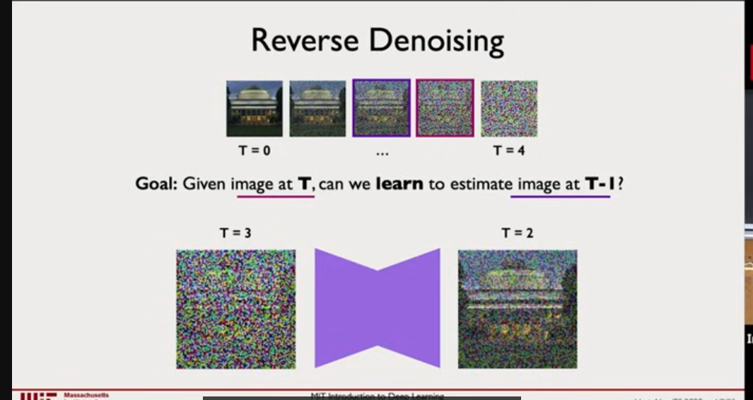
Forward process: Add noise to a real data sample gradually until it becomes pure noise.

Reverse process: Train a neural network to denoise step by step, predicting the previous less-noisy version. so we feed the noisy version and try to predict the previous noisy version and so on

Loss: Mean Squared Error (MSE) between predicted denoised image and actual slightly less noisy image.

Sampling (Generation): - Start from random noise. - Apply the trained denoising network iteratively → gradually reconstruct a realistic sample. Advantages: - High fidelity outputs. - Stable training. - Can generate diverse outputs (avoids mode collapse). - Works across domains: images, video, audio, molecular structures.

Real-World Impact: - Text-to-image generation (DALL·E, Stable Diffusion). - Molecular design & protein folding in life sciences. - Image/video super-resolution, inpainting, denoising.

Generative Adversarial Networks (GANs)

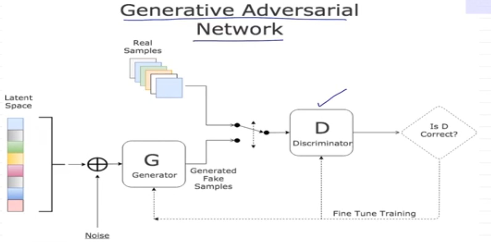
Generator (G):

Takes random noise z as input
Outputs fake data G(z)
Goal: Fool the discriminator
Wants to minimize the value function

Discriminator (D):

Takes data (real or fake) as input
Outputs a probability: D(x) = “Is this real?”
Goal: Correctly classify real vs fake
Wants to maximize the value function

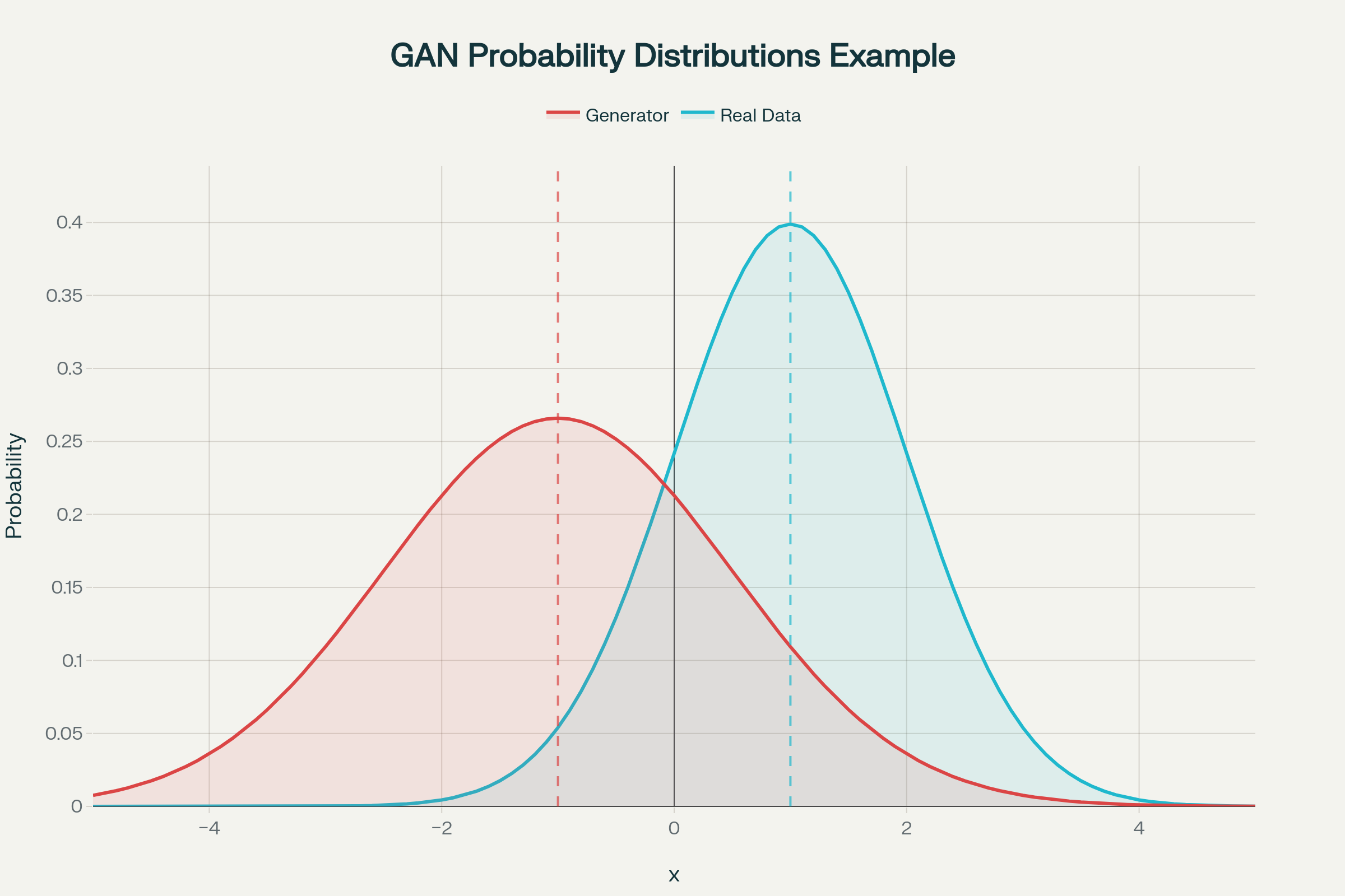
we need to make the genrator to match with real data probablity distribution

Generative Adversarial Networks

Table of Contents

Discriminative Models

Generative Models

Deep Generative Models

Autoencoders

Variational Autoencoders (VAEs)

Concrete examples

kullback leibler divergence

My understanding

1. The Input Layer

2. The Encoder (Dimensionality Reduction)

3. The Reparameterization Trick (The Magic Step)

4. The Decoder (Reconstruction)

5. The Output & Loss

Summary Table: Data Transformation

A. Reconstruction Loss (The “Realism” Term)

B. KL Divergence (The “Organization” Term)

VAE: How Distributions Work Under The Hood

PART 1: Regular Autoencoder (Point Mapping)

What Actually Happens

PART 2: VAE Encoder (Distribution Mapping)

Architecture Change

Concrete Computation

Why log(σ²) Instead of σ Directly?

PART 3: The Sampling Operation

What Distribution Actually Means

Sampling: Drawing from Distribution

PART 4: Reparameterization Trick (Deep Dive)

The Problem: Gradients Through Randomness

The Solution: Reparameterization

Detailed Gradient Calculation

PART 5: Complete Forward-Backward Pass

Full Numerical Example

Forward Pass

Backward Pass

PART 6: Why This Creates Distributions

Computational Perspective

What “Distribution” Means Computationally

Training Effect

PART 7: The Mathematical Guarantee

Why KL Loss Creates Smooth Space

Numerical Example of KL Penalty

Summary: Under The Hood

Resources

Diffusion Models

Generative Adversarial Networks (GANs)

Resources

Graph View