RNN (Recurrent Neural Network)

Forward Propagation in an RNN

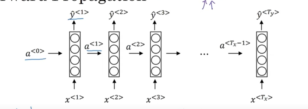
In a Recurrent Neural Network (RNN), forward propagation is the process where the network takes an input sequence, passes it through its layers, and produces an output sequence. Here’s how it works:

Basic RNN Setup

• Input data: At each time step, you have an input $x^{(t)}$, which is a vector (could be a word, a number, etc.).
• Hidden state: The RNN has a hidden state $a^{(t)}$, which “remembers” information from previous time steps. This hidden state is updated at each time step based on the previous hidden state and the current input.
• Output: The RNN also produces an output ${\hat{y}}^{(t)}$ at each time step.

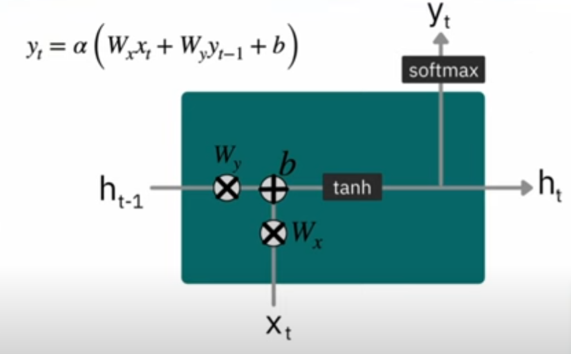
The Key Equations in RNN Forward Propagation:

1. Hidden State Update

At each time step $t$, the hidden state $a^{(t)}$ is updated using the previous hidden state $a^{(t-1)}$ and the current input $x^{(t)}$.

$$a^{(t)}=g(W_{aa}\cdot a^{(t-1)}+W_{ax}\cdot x^{(t)}+b_a)$$

Here:

• $W_{aa}$: Weight matrix that connects the previous hidden state $a^{(t-1)}$ to the current hidden state.
• $W_{ax}$: Weight matrix that connects the current input $x^{(t)}$ to the current hidden state.
• $b_a$: Bias term added to the hidden state calculation.
• $g$: Activation function (like tanh or ReLU) applied to the weighted sum. It helps the RNN model learn complex relationships.

What’s Happening Here:

• The previous hidden state $a^{(t-1)}$ contains information about the past (the history), and we combine it with the current input $x^{(t)}$ to compute the new hidden state $a^{(t)}$.
• The weights $W_{aa}$ and $W_{ax}$ control how much of the previous state and the current input should influence the new hidden state.
• The activation function $g$ introduces non-linearity, which helps the model learn more complex patterns.

2. Output Calculation

Once we compute the hidden state $a^{(t)}$ for a given time step, we then calculate the output ${\hat{y}}^{(t)}$ at that time step.

$${\hat{y}}^{(t)}=g(W_{ya}\cdot a^{(t)}+b_y)$$

Here:

• $W_{ya}$: Weight matrix that connects the hidden state $a^{(t)}$ to the output.
• $b_y$: Bias term for the output.
• $g$: Activation function (like softmax for classification tasks or sigmoid for binary classification).

What’s Happening Here:

• The output ${\hat{y}}^{(t)}$ is calculated by applying the weight matrix $W_{ya}$ to the current hidden state $a^{(t)}$.
• The output layer’s activation function $g$ ensures that the output has the right scale (e.g., for classification, softmax gives probabilities).

Vector repersentation of Hidden state and output

Hidden State Update:

$$a^{(t)}=g(W_{aa}\cdot a^{(t-1)}+W_{ax}\cdot x^{(t)}+b_a)$$

In vector form:

• we combine the weight and a to single vector

$$a^{(t)}=g\left(\left[\begin{array}{cc}{W}_{aa}& W_{ax}\end{array}\right]\cdot \left[\begin{array}{c}{a}^{(t-1)}\\ x^{(t)}\end{array}\right]+b_a\right)$$

Output Calculation:

$${\hat{y}}^{(t)}=g(W_{ya}\cdot a^{(t)}+b_y)$$

In vector form:

$${\hat{y}}^{(t)}=g\left(W_{ya}\cdot a^{(t)}+b_y\right)$$

Back Propagation in an RNN

Forward pass: First, we compute the output using the forward propagation formulas.

Loss function: After computing the predicted output y^(t)\hat{y}^{(t)}y^​(t), the loss is calculated (e.g., cross-entropy loss). This loss is then propagated back through the network.

Backward pass: Compute the gradients of the weights with respect to the loss. This requires applying the chain rule for each time step ttt in the sequence. The gradients are then used to update the weights.

Backpropagation Through Time (BPTT) in RNN

In an RNN, backpropagation is the process used to optimize the weights by adjusting them based on the error between the predicted output ${\hat{y}}^{(t)}$ and the actual output $y^{(t)}$. The idea is to propagate the error backward through the network, layer by layer, to update the weights. This process can be extended to sequences, and that’s called Backpropagation Through Time (BPTT).

Loss function

We calculate the loss to see how wrong our predictions are. Typically, for classification problems, we use cross-entropy loss:

$L^{(t)}=-y^{(t)}\log ({\hat{y}}^{(t)})-(1-y^{(t)})\log (1-{\hat{y}}^{(t)})$

Where:

• $L^{(t)}$ is the loss at time step $t$.
• $y^{(t)}$ is the actual value (ground truth).
• ${\hat{y}}^{(t)}$ is the predicted output from the RNN.

1. Gradient of the Output Layer:

For each time step $t$, the gradient of the loss with respect to the predicted output ${\hat{y}}^{(t)}$ is computed.

$$\frac{\partial L^{(t)}}{\partial {\hat{y}}^{(t)}}={\hat{y}}^{(t)}-y^{(t)}$$

This is the difference between the predicted output and the actual output, which will be propagated back to update the weights.

2. Gradient of the Hidden Layer:

Now, we need to compute the gradient of the loss with respect to the hidden state $a^{(t)}$. To do this, we use the chain rule, considering that the hidden state $a^{(t)}$ is influenced by the previous hidden state $a^{(t-1)}$ and the current input $x^{(t)}$.

We compute the gradient of the loss at each time step with respect to $a^{(t)}$:

$$\frac{\partial L^{(t)}}{\partial a^{(t)}}=\frac{\partial L^{(t)}}{\partial {\hat{y}}^{(t)}}\cdot \frac{\partial {\hat{y}}^{(t)}}{\partial a^{(t)}}$$

Since the output ${\hat{y}}^{(t)}$ is a function of $a^{(t)}$, we apply the chain rule:

$$\frac{\partial {\hat{y}}^{(t)}}{\partial a^{(t)}}=W_{ya}$$

Thus, the gradient for the hidden state becomes:

$$\frac{\partial L^{(t)}}{\partial a^{(t)}}=({\hat{y}}^{(t)}-y^{(t)})\cdot W_{ya}$$

3. Gradient of the Hidden State Update:

Now, we compute the gradient of the loss with respect to the weights $W_{aa}$, $W_{ax}$, and the bias $b_a$ involved in the update rule for the hidden state $a^{(t)}$.

To do this, we apply the chain rule considering that the hidden state at time step $t$ depends on the previous hidden state $a^{(t-1)}$ and the input $x^{(t)}$.

We start by computing the gradient with respect to $a^{(t-1)}$:

$$\frac{\partial L^{(t)}}{\partial a^{(t-1)}}=\frac{\partial L^{(t)}}{\partial a^{(t)}}\cdot \frac{\partial a^{(t)}}{\partial a^{(t-1)}}$$

The hidden state update equation is:

$$a^{(t)}=g(W_{aa}\cdot a^{(t-1)}+W_{ax}\cdot x^{(t)}+b_a)$$

Therefore, the derivative with respect to $a^{(t-1)}$ is:

$$\frac{\partial a^{(t)}}{\partial a^{(t-1)}}=W_{aa}\cdot g^{\prime }(W_{aa}\cdot a^{(t-1)}+W_{ax}\cdot x^{(t)}+b_a)$$

Where $g^{\prime }$ is the derivative of the activation function.

4. Updating the Weights and Biases:

The gradients computed above allow us to update the weights using gradient descent. The updates for the weights and biases at time step $t$ are as follows:

• For the weights $W_{ya}$ between the hidden state and the output:

$$W_{ya}\leftarrow W_{ya}-\eta \frac{\partial L^{(t)}}{\partial W_{ya}}$$

Where $\eta$ is the learning rate.

• Similarly, for the weights $W_{aa}$ and $W_{ax}$, and the biases $b_a$ and $b_y$, the gradients are computed and the weights are updated accordingly.

Question i have is

• i need to write this one step by hand one time to fully understand

Types of RNN

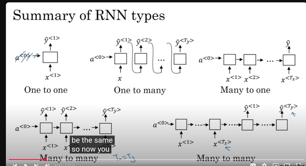
1. One to One

• Diagram: One input $x^{<1>}$ gives one output ${\hat{y}}^{<1>}$.
• Example: A regular feedforward neural network (no sequence).
• Use case: Basic classification or regression tasks where input and output are single data points (e.g., image classification).

2. One to Many

• Diagram: One input $x$ produces many outputs ${\hat{y}}^{<1>},{\hat{y}}^{<2>},...,{\hat{y}}^{<T_y>}$.
• Example: Image captioning.
• Explanation: You give one input (an image), and the model generates a sequence of outputs (a sentence describing the image).
• Why use? When a single input corresponds to multiple outputs over time.

3. Many to One

• Diagram: Many inputs $x^{<1>},x^{<2>},...,x^{<T_x>}$ produce one output $\hat{y}$.
• Example: Sentiment analysis.
• Explanation: The model reads a whole sequence (like a sentence) and outputs one single prediction (e.g., positive or negative sentiment).
• Why use? When you want to summarize or classify an entire input sequence with one output.

4. Many to Many (Equal length inputs and outputs)

• Diagram: Many inputs $x^{<1>},x^{<2>},...,x^{<T_x>}$ produce many outputs ${\hat{y}}^{<1>},{\hat{y}}^{<2>},...,{\hat{y}}^{<T_y>}$, where $T_x=T_y$.
• Example: Part-of-speech tagging.
• Explanation: The model reads a sequence and outputs a sequence of the same length (e.g., each word gets tagged).
• Why use? When you want to generate an output for every input element.

5. Many to Many (Different length inputs and outputs)

• Diagram: Many inputs $x^{<1>},x^{<2>},...,x^{<T_x>}$ produce many outputs ${\hat{y}}^{<1>},{\hat{y}}^{<2>},...,{\hat{y}}^{<T_y>}$, but $T_x\ne T_y$.

• Example: Machine translation (English sentence to French sentence).

• Explanation: Input and output sequences are both variable length but not necessarily equal.

• Why use? For tasks where input and output lengths differ but both are sequences.

Building Next word prediction model

Given a sequence of words, we want the RNN to learn how to predict the next word.

For example:

“Cats average 15 hours of sleep a day.”

We want the model to learn to predict:

• After “Cats” → “average”
• After “Cats average” → “15”
• After “Cats average 15” → “hours”
• Finally, predict the end of sentence: <EOS>

1. Inputs and Outputs in Time Steps

Each time step in an RNN receives:

• Input $x^{<t>}$: A word (converted into a word vector).
• Hidden state $a^{<t>}$: Stores memory from the previous time steps.
• Output ${\hat{y}}^{<t>}$: The prediction (probability distribution over vocabulary for the next word).

2. First Time Step $t=1$

• $a^{<0>}=0$: Initial hidden state is zero.
• $x^{<1>}=0$: The special “start-of-sentence” token.
• Output: ${\hat{y}}^{<1>}$: Predicted probability of first word.
• Example: P(cats), P(dogs), P(the), etc.
• Suppose the correct word is “Cats” → loss compares ${\hat{y}}^{<1>}$ to “Cats”

3. Second Time Step $t=2$

• $x^{<2>}=y^{<1>}=\text{“Cats”}$: Feed previous actual word.
• $a^{<2>}$: Computed from $x^{<2>}$ and $a^{<1>}$
• Output ${\hat{y}}^{<2>}$: Predicts the next word (like “average”)

4. Third Time Step $t=3$

• $x^{<3>}=y^{<2>}=\text{“average”}$
• Hidden state updates to $a^{<3>}$
• Output ${\hat{y}}^{<3>}$: Predicts “15”

5. This Continues Until <EOS>

• Eventually, it predicts the final word → <EOS> (end of sentence)

Loss Function

The loss measures how well the model’s predicted word distribution matches the actual next word.

For a single time step:

$${\mathcal{L}}^{<t>}=-\sum _i{y}_i^{<t>}\log ({\hat{y}}_i^{<t>})$$

• This is cross-entropy loss
• $y_i^{<t>}$ is the true word (one-hot encoded)
• ${\hat{y}}_i^{<t>}$ is the predicted probability for that word

For the whole sentence:

$$\mathcal{L}=\sum _{t=1}^T{\mathcal{L}}^{<t>}$$

• Sum the loss over every word in the sequence.

In Training vs. Inference

During training:

• The input at each step is the true previous word (teacher forcing).
• So: $x^{<t>}=y^{<t-1>}$

During inference (prediction):

• The input is the model’s own predicted word from the previous step:
• $x^{<t>}={\hat{y}}^{<t-1>}$

Vanishing Gradients

The vanishing gradient problem occurs when the gradient values become extremely small during backpropagation, specifically as information flows backward through many layers or time steps. This is similar to what happens in very deep standard neural networks

Gated Recurrent Units

GRUs are a modification to the basic RNN hidden layer designed to address the vanishing gradient problem and improve the capture of long-range connections

we will have two new state

• Reset Gate: Determines how much of the previous memory should be ignored when computing the candidate state.
• Update Gate: Controls how much of the new candidate state should replace the old memory.

Vector notation

Candidate Hidden State: ${\tilde{c}}^{(t)}=\tanh (W_c[{\Gamma }_r\cdot c^{(t-1)},x^{(t)}]+b_c)$

Update Gate: ${\Gamma }_u=\sigma (W_u[c^{(t-1)},x^{(t)}]+b_u)$

Reset Gate: ${\Gamma }_r=\sigma (W_r[c^{(t-1)},x^{(t)}]+b_r)$

Final Hidden State: $c^{(t)}={\Gamma }_u\cdot {\tilde{c}}^{(t)}+(1-{\Gamma }_u)\cdot c^{(t-1)}$

GRU_RNN

Exploding Gradients

Exploding gradients are the opposite problem, where gradients grow exponentially during backpropagation

large gradients can cause neural network parameters to become extremely large and unstable, leading to numerical overflow (e.g., resulting in “Not a Number” or NaN values)

Exploding gradients are generally easier to detect and address than vanishing gradients. The common solution is gradient clipping, which involves rescaling gradient vectors if their magnitude exceeds a certain threshold

LSTM

In a vanilla RNN the recurrence:

$$h_t=\tanh (W{x}_t+U{h}_{t-1}+b)$$

When we train through many time steps, gradients get multiplied repeatedly by weights and activations.

• If the multipliers < 1 → gradients shrink → vanishing gradient.

• If multipliers > 1 → gradients blow up → exploding gradient.

Result:

• RNNs can’t remember dependencies from far back in the sequence.
• They “forget” old context.

“How do we let a neural network decide what to remember and what to forget over long time scales?”

The answer: give the network a separate memory track (called the cell state $c_t$) that can carry information along mostly unchanged, with small updates.

Think of it like:

• $h_t$ = short-term working memory.
• $c_t$ = long-term storage, guarded by gates.

The gates in LSTM

An LSTM cell introduces three main gates (all are tiny neural nets with sigmoid activations, values between 0 and 1):

1. Forget gate: $f_t=\sigma (W_f{x}_t+U_f{h}_{t-1}+b_f)$

Decides which parts of the old cell state to keep vs. forget.

(If $f_t=0$, that info is erased; if $f_t=1$, it’s kept.)

2. Input gate: $i_t=\sigma (W_i{x}_t+U_i{h}_{t-1}+b_i)$

Decides which new info should enter memory.

Alongside, a candidate memory is created: ${\tilde{c}}_t=\tanh (W_c{x}_t+U_c{h}_{t-1}+b_c)$

3. Update cell state: $c_t=f_t\odot c_{t-1}+i_t\odot {\tilde{c}}_t$

(Forget some of the past, add some of the new.)

4. Output gate:$o_t=\sigma (W_o{x}_t+U_o{h}_{t-1}+b_o)$

Then the hidden state is updated as:$h_t=o_t\odot \tanh (c_t)$

So the full LSTM cell has: forget gate, input gate, output gate, and a cell state pipeline.

Unfolding an LSTM

Like an RNN, you still unfold it over time:

x1 → [LSTM Cell] → h1, c1

x2 → [LSTM Cell] → h2, c2

x3 → [LSTM Cell] → h3, c3

But now, each cell has two highways:

• The hidden state $h_t$ (short-term).

• The cell state $c_t$ (long-term).

The gates let information survive many steps without vanishing, because $c_t$ can be passed forward almost unchanged if gates allow it.

FLow

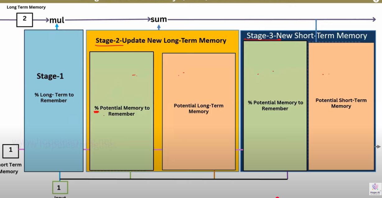
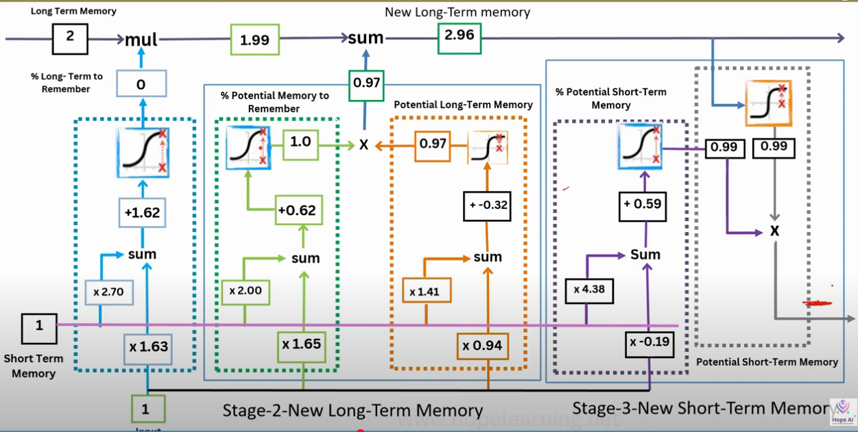
Stage 1: Forgetting (Filter Old Long-Term Memory)

• Input: previous cell state ($c_{t-1}$) = long-term memory up to now.
• Gate: Forget gate $f_t$.
• Operation: multiply old memory by $f_t$.
  • If $f_t=1$: keep everything.
  • If $f_t=0$: erase completely.
• Usually, it’s a fraction in between.

Interpretation: “How much of the past memory should I carry forward?”

Stage 2: Updating the New Long-Term Memory

This is where new info is injected. Two sub-parts happen:

1. Candidate memory (${\tilde{c}}_t$)
   • Computed from current input $x_t$ + previous short-term memory ($h_{t-1}$).
   • Tanh squashes it into range $[-1,1]$.
   • Represents new knowledge I could add.
2. Input gate ($i_t$)
   • Decides how much of this candidate memory should enter.
   • Works like a filter:
   • If $i_t=0$, ignore new info.
   • If $i_t=1$, accept fully.
3. Combine $c_t=f_t\cdot c_{t-1}+i_t\cdot {\tilde{c}}_t$
   • Old memory (partially kept) + New candidate info (partially added).
   • This gives the updated long-term memory.

Interpretation: “Erase some old stuff, add some new stuff, keep the rest.”

Stage 3: Producing the Short-Term Memory (Hidden State)

Now we decide what to output for this step:

1. Output gate ($o_t$)

   • Looks at $x_t$ + $h_{t-1}$.
   • Decides which parts of memory to reveal.

2. Short-term memory $h_t$ $h_t=o_t\cdot \tanh (c_t)$

   • Apply tanh to long-term memory (compress range).
   • Multiply by output gate (select relevant parts).

Interpretation: “What part of my internal memory should I make visible right now as my working memory?”

Imagine you’re a student carrying a notebook through a lecture series:

• Stage 1 (Forget gate): Before a new class, you erase some irrelevant notes.

• Stage 2 (Input gate + candidate memory): You write down new things the teacher says, but only if they seem important.

• Stage 3 (Output gate): When asked a question, you don’t read out your entire notebook you selectively share the part that matters.

GRU

BiLSTM

A Bidirectional Long Short-Term Memory (BiLSTM) is a type of recurrent neural network (RNN) architecture that is used to process sequential data. It extends the standard Long Short-Term Memory (LSTM) model by introducing the concept of bidirectionality, allowing the model to have both forward and backward information about the sequence.

The architecture of a BiLSTM is as follows:

1. Input Layer: Takes the input sequence.
2. Embedding Layer: Converts the input tokens to dense vectors (embeddings).
3. Forward LSTM Layer: Processes the input sequence from start to end.
4. Backward LSTM Layer: Processes the input sequence from end to start.
5. Concatenation Layer: Combines the outputs from both the forward and backward LSTM layers.
6. Dense Layer: Optional layer(s) for further processing.
7. Output Layer: Produces the final predictions.

Resources

• https://colah.github.io/posts/2015-08-Understanding-LSTMs/

• https://www.kaggle.com/code/fareselmenshawii/rnn-from-scratch

• https://research.google/blog/a-neural-network-for-machine-translation-at-production-scale/

• https://www.iamtk.co/building-a-recurrent-neural-network-from-scratch-with-python-and-mathematics

• https://blog.otoro.net/2017/01/01/recurrent-neural-network-artist/

• Yann LeCun’s Deep Learning Course

TO check

• VISUALIZING AND UNDERSTANDING RECURRENT NETWORKS

  • https://arxiv.org/pdf/1506.02078

• Multilingual Machine Translation with Large Language Models: https://arxiv.org/pdf/2304.04675

• On the difficulty of training Recurrent Neural Networks

• https://github.com/dennybritz/rnn-tutorial-rnnlm

• https://dennybritz.com/posts/wildml/recurrent-neural-networks-tutorial-part-2/

• https://iamtrask.github.io/2015/11/15/anyone-can-code-lstm/

• https://victorzhou.com/blog/intro-to-rnns/

• https://arxiv.org/pdf/1909.09586

• https://chatgpt.com/c/68afc6d1-9590-8322-8f05-d234397761aa

• https://cs231n.github.io/neural-networks-case-study/