
Liquid Time-Constant Networks (LTCs) are a type of time-continuous recurrent neural network inspired by efficient biological systems like the C. elegans worm, which performs complex survival tasks with just 302 neurons. Unlike massive deep learning models, LTCs use fewer neurons but achieve high expressivity through dynamic, input-dependent time constants
Researchers, including Ramin Hasani at MIT, drew from the nematode worm C. elegans, whose simple nervous system enables learning, navigation, and adaptation despite its tiny size. This contrasts with human brains (about 86 billion neurons) and modern AI models (billions of parameters), prompting designs for compact, adaptive networks that mimic biological efficiency without scaling up.
The intuition behind Liquid Time-Constant (LTC) Networks lies in mimicking how biological neurons adapt their response speed like slowing down for steady signals or speeding up for urgent ones instead of using fixed rules. This “liquid” flexibility lets a small network handle complex, changing data efficiently, much like the C. elegans worm’s 302 neurons manage survival tasks without massive scale
At the core of Liquid Neural Networks lies an exciting scientific concept: Liquid Time-Constant (LTC) models. These models are inspired by how neurons in our brains work—not just reacting to stimuli, but changing their behavior based on time, context, and past experience.
Let’s simplify it.
What Is a Time Constant?
In neuroscience, neurons don’t respond to signals instantly. They integrate inputs over time and adjust how quickly they respond depending on the situation. This “delay” or adaptability is called the time constant. It’s what helps the brain stay calm in some situations and react fast in others.
Liquid Neural Networks mimic this behavior.
How Do Liquid Time-Constant Models Work?
In an LNN, each neuron has its own time constant, and here’s the twist—it’s not fixed. Instead, it changes based on the incoming data.
That means:
- The speed of response varies depending on the input.
- The output changes not just based on the current input, but also on how fast or slow that input arrived.
- The network’s behavior is context-sensitive and time-aware.
This is different from traditional RNNs or LSTMs, which use fixed rules for how memory and time are handled. In LNNs, the response itself is a dynamic equation, not a static function.
What if the network kept a little memory variable let’s call it x that it updates every moment?
Think of x like water in a tank. Right now it holds some amount. Every second, two things happen:
- Some water leaks out naturally (the tank has a small hole)
- New water pumps in based on the current input
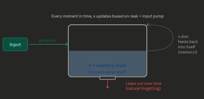
This is the core idea behind all recurrent networks. The water level x right now carries memory of everything that happened before.
A normal recurrent network has a fixed leak rate. The water always drains at the same speed no matter what.
An LTC says: what if the valve speed changes depending on what’s happening right now?
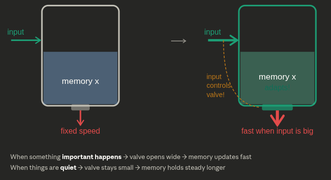
That self-adjusting valve speed is called the liquid time-constant. That’s literally where the name comes from — “liquid” because it’s fluid, it changes.
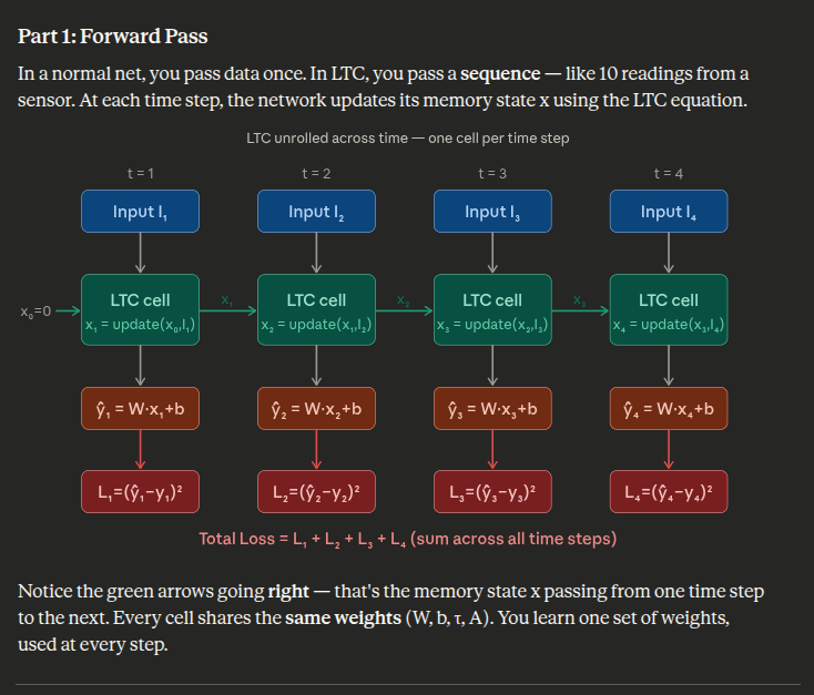
1 Step 1 — Natural decay (if nothing else happened)
dx/dt = −x/τ = −10.0 / 2.0 = -5.0000
x would become: 10.0 + 0.1 × -5.0000 = 9.5000
↳ Just forgetting. No input yet.
2 Step 2 — We have a raw input I = 8.0
Raw input pushes back: dx/dt = −x/τ + I = -5.000 + 8.0 = 3.0000
↳ Better, but input goes in raw. We need to learn from it.
3 Step 3 — Pass through mini neural net → f
z = w·x + w·I + b = 0.5×10.0 + 0.5×8.0 + 0.0 = 9.0000
f = tanh(9.0000) = 1.000000
↳ f is between −1 and +1. Right now: strong signal.
4 Step 4 — Compute liquid τ_system using f
τ_sys = τ / (1 + τ×|f|) = 2.0 / (1 + 2.0×1.0000)
= 2.0 / 3.0000 = 0.666667
↳ Base τ was 2.0, now it’s 0.6667 — faster reaction.
5 Step 5 — Full LTC equation
Pull: −(1/τ + f)·x = −(0.500 + 1.0000) × 10.0 = -15.0000
Push: f·A = 1.0000 × 5.0 = 5.0000
dx/dt = -15.0000 + 5.0000 = -10.0000
↳ x is moving down toward A.
6 Step 6 — Fused solver: compute x_new in one shot
numerator = x + Δt×f×A = 10.0 + 0.1×1.0000×5.0 = 10.500000
denominator = 1 + Δt×(1/τ+f) = 1 + 0.1×(0.500+1.0000) = 1.150000
x_new = 10.5000 / 1.1500 = 9.130435
↳ Memory updated: 10.0 → 9.1304
The whole thing in one breath: you start with memory x, pass it and the input through a mini neural net to get f, use f to shrink τ into a liquid τ_system, then use that to compute how fast x moves toward the target A. Step 6 is just the computer-friendly way to do step 5 in one calculation instead of tiny steps.
LFM
LFM2 = Liquid Foundation Model 2. It’s a family of small-but-smart AI language models designed to run fast on your phone or laptop
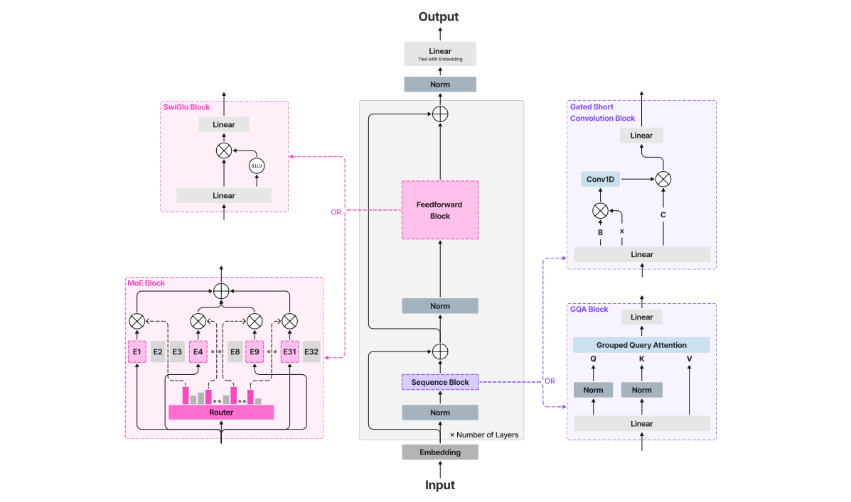
Replace most “expensive” attention layers with a cheaper operation called a gated short convolution, keep a few attention layers for the hard tasks, and train with clever tricks to punch above their weight class.
The Architecture (the big idea)
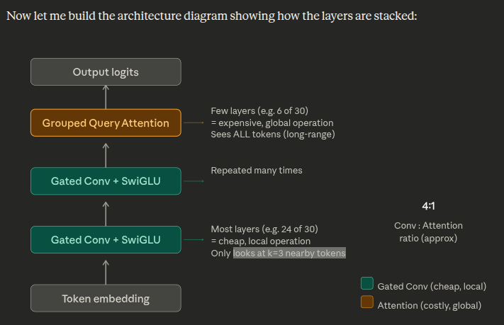
A standard Transformer uses attention in every layer. Attention is powerful but expensive. LFM2’s key insight: most layers don’t need it. Here’s what a standard layer vs LFM2 layer looks like:
Standard Transformer layer
y = Attention(x) + FFN(x)
Attention computes relationships between every pair of tokens. If you have 1000 tokens, that’s 1000×1000 = 1M comparisons. Very slow on phones.
LFM2 layer (most layers)
y = GatedConv(x) + SwiGLU(x)
The gated conv only looks at a small window of nearby tokens (kernel size k=3). Much cheaper! Attention is used in only a few layers where it’s truly needed.
The Gated Short Convolution the math
This is the core operation. Given an input sequence h (shape: L tokens × d dimensions):
Step 1: (B, C, h̃) = Linear(h) ← split into 3 parts
Step 2: y = B ⊙ h̃ ← element-wise multiply (gate!)
Step 3: z = Conv₁D_k(y) ← 1D convolution, kernel size k=3
Step 4: o = Linear_out(C ⊙ z) ← gate again, then project out
The ⊙ symbol means element-wise multiply. B and C are “gates” — they act like valves that control how much of the signal flows through. This is similar to how an LSTM uses forget/input gates, but much simpler and faster.
The convolution Conv₁D_k is depthwise — each channel is filtered independently, which is much cheaper than a full convolution.
Grouped Query Attention (GQA)
Standard multi-head attention stores separate Key and Value matrices for every attention head. GQA shares K and V across groups of heads, dramatically cutting memory:
Standard attention (MHA)
Q: 32 heads × d
K: 32 heads × d ← big!
V: 32 heads × d ← big!
Each head has its own K,V stored in memory (KV cache).
LFM2 GQA (32Q heads, 8KV groups)
Q: 32 heads × d
K: 8 groups × d ← 4× smaller!
V: 8 groups × d ← 4× smaller!
Every 4 query heads share one K,V pair. Same expressiveness, 4× less memory.
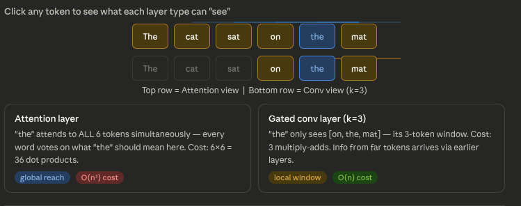
Attention is like a phone call — any token can directly ask any other token “what are you about?” Convolution is like a game of telephone — token 1 whispers to token 2, token 2 carries that forward and whispers to token 3, and by token 20 the message has traveled far. Phone calls are expensive (you have to dial everyone). Telephone is cheap but takes more rounds.
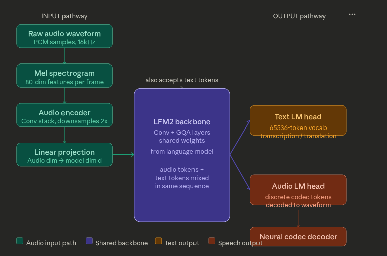
LFM2-Audio
Stage 1 — Raw audio to mel spectrogram
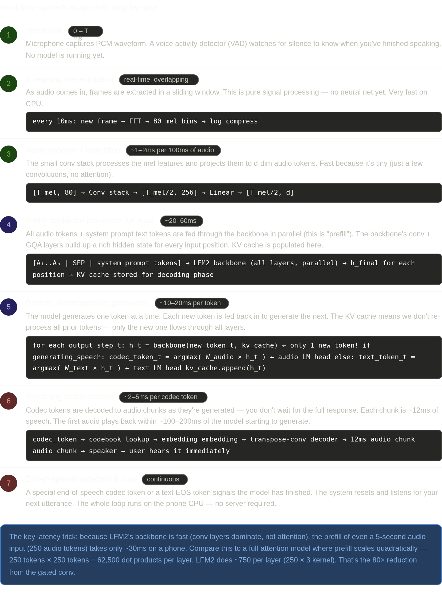
Your microphone produces a continuous waveform: a series of pressure values (PCM samples) at 16,000 samples per second. The model can’t eat raw samples there are too many and they contain a lot of redundancy. So first, they’re converted to a mel spectrogram.
Step 1: Slice waveform into overlapping frames frame_size = 400 samples = 25ms (a short window of sound) hop_size = 160 samples = 10ms (step between frames) → 1 second of audio = 100 frames Step 2: Apply FFT to each frame FFT(frame) → complex spectrum of frequencies present Step 3: Map to mel scale (log-spaced, matches human hearing) mel_bank = 80 triangular filters × spectrum → each frame becomes a vector of 80 numbers → these numbers = “how much energy at each frequency band” Step 4: Log compression mel_feat = log(mel_bank + 1e-9) ← makes quiet sounds visible too Result: audio (T seconds) → matrix of shape [T×100, 80] e.g. 3 seconds → [300 frames, 80 mel bins]
Why mel scale? It’s logarithmic in frequency, matching how the human ear works. The difference between 100Hz and 200Hz sounds like the same “amount” as 1000Hz and 2000Hz — both are one octave. The model learns in terms of perceptual similarity, not raw Hz.
Stage 2 — Audio encoder (Conv stack)
The mel features are still pretty high-frequency (100 frames/second). The audio encoder uses a small stack of 1D convolutions to compress them — downsampling by 2× — so the backbone sees 50 audio tokens per second instead of 100. This is critical for speed.
Input: mel features shape = [T_frames, 80] Audio encoder (small Conv stack): Conv1D(80 → 256, kernel=3, stride=1) → compress channels Conv1D(256 → 256, kernel=3, stride=2) → downsample by 2× ← key! Conv1D(256 → 256, kernel=3, stride=1) → refine + Layer norm + GELU activations Output: audio_feats shape = [T_frames/2, 256]
The stride=2 in the middle conv means every output frame summarises 2 input frames. Information isn’t lost — it’s compressed. 1 second of speech goes from 100 frames → 50 audio tokens entering the backbone.
Stage 3 — Linear projection into model space
The backbone expects vectors of size d (e.g. 2048 for LFM2-2.6B). The audio encoder outputs 256-dim vectors. A simple learned linear map bridges the two:
audio_token = Linear(audio_feat) = W_proj × audio_feat + b_proj where: W_proj shape = [d_model, 256] e.g. [2048, 256] b_proj shape = [d_model] Result: each audio frame is now a d-dimensional vector, exactly the same shape as a text token embedding. → Audio tokens and text tokens become interchangeable.
50 audio tokens per second entering backbone
shape as text token — no special routing needed
This is the elegance of the design: after projection, the backbone literally cannot distinguish “this was audio” from “this was text” by shape alone. They’re all just vectors flowing through the same layers.
- LFM2-Extract – A 350M and 1.2B multilingual models for data extraction from unstructured text, like turning invoice emails into JSON objects.
- LFM2‑350M‑ENJP‑MT – A 350M model for bidirectional English ↔ Japanese translation.
- LFM2‑1.2B‑RAG – A 1.2B model optimized for long‑context question answering in RAG pipelines.
- LFM2‑1.2B‑Tool – A 1.2B model built for function calling and agentic tool use.
- LFM2‑350M‑Math – A 350M reasoning model for solving mathematical problems.
- Luth-LFM2 – An additional community-driven series of French fine-tunes to enable general-purpose assistants for on-device chat.