Voice LLM

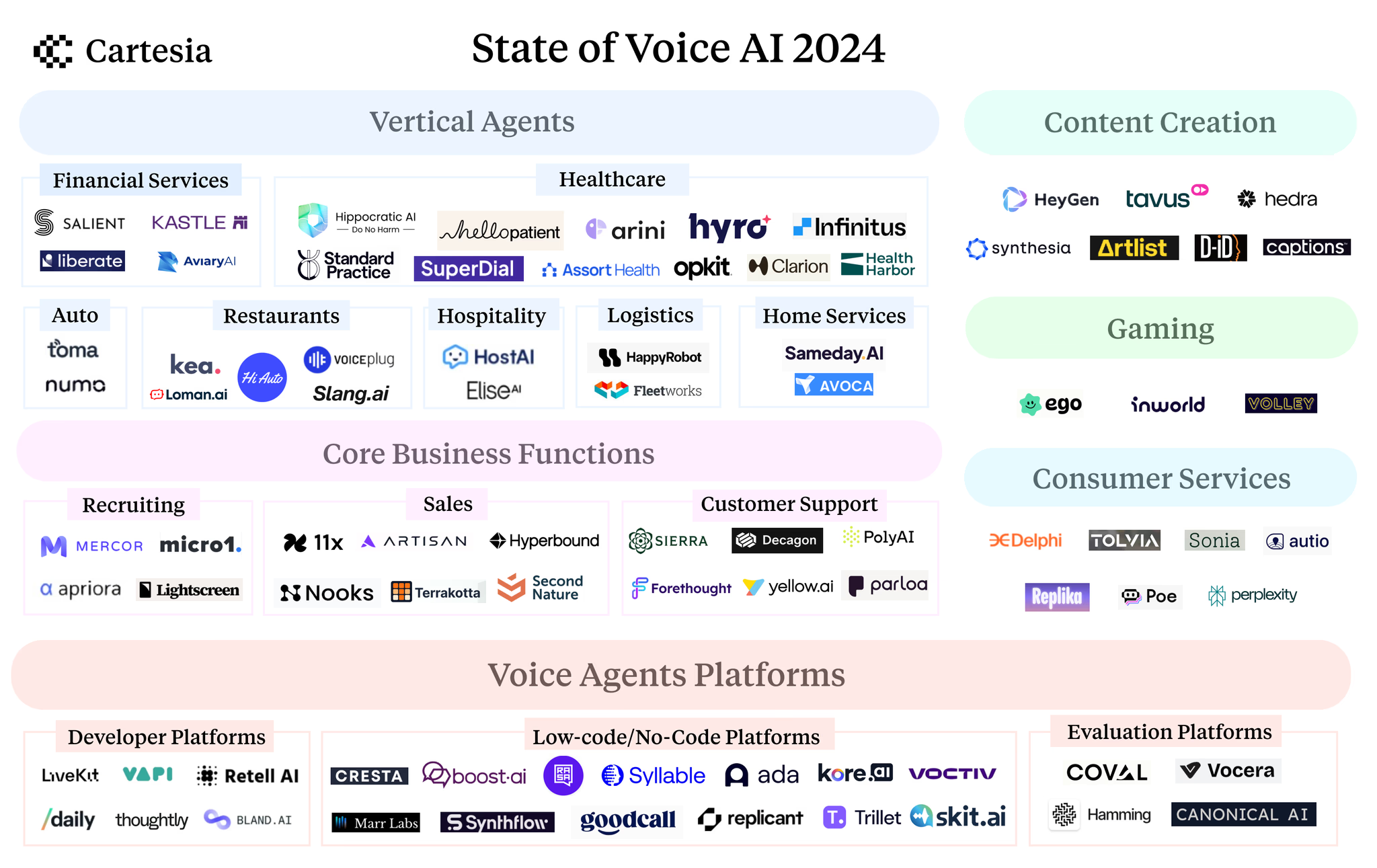
https://www.resemble.ai/chatterbox/

https://www.bolna.ai/ for india voice agents

https://inworld.ai/

FlashLabs Chroma 1.0

https://www.neuphonic.com/text-to-speech https://gradium.ai/ https://kyutai.org/ https://www.pyannote.ai/ https://pareto.ai/

https://huggingface.co/nvidia/personaplex-7b-v1 (similar to moshi speact to speach model)

https://waywithwords.net/

• https://narilabs.org/ # Open-Source TTS AI by Nari Labs

https://github.com/kyutai-labs/moshi

https://github.com/fishaudio/fish-speech https://kokorottsai.com/#google_vignette https://github.com/fishaudio/fish-speech https://github.com/huggingface/parler-tts

https://www.google.com/search?q=SoTA+open+source+TTS&oq=SoTA+open+source+TTS&gs_lcrp=EgZjaHJvbWUqBggAEEUYOzIGCAAQRRg7Mg0IARAAGIYDGIAEGIoFMgoIAhAAGIAEGKIEMgoIAxAAGIAEGKIEMgoIBBAAGIAEGKIEMgYIBRBFGD0yBggGEEUYPDIGCAcQRRg80gEHMzgxajBqMagCALACAA&sourceid=chrome&ie=UTF-8

• https://github.com/canopyai/Orpheus-TTS

  • https://huggingface.co/isaiahbjork/orpheus-3b-0.1-ft-Q4_K_M-GGUF

• https://huggingface.co/Qwen/Qwen2.5-Coder-7B-Instruct

https://github.com/vllm-project/aibrix

https://www.zyphra.com/

• https://www.trillet.ai/ (nice

https://github.com/KittenML/KittenTTS?ref=dailydev https://cartesia.ai/

https://github.com/open-mmlab/Amphion/tree/main/models/tts/maskgct

• https://github.com/kyutai-labs/hibiki?tab=readme-ov-file

https://ai-coustics.com/ Voice AI that stands out from the noise

https://www.sesame.com/

• https://huggingface.co/learn/audio-course/chapter1/audio_data

Need to check

• https://github.com/k2-fsa/ZipVoice
• https://github.com/KoljaB/RealtimeTTS/blob/master/RealtimeTTS/engines/zipvoice_engine.py

https://www.fluents.ai/

indian voice

• https://www.gnani.ai/

HIstory

A key breakthrough in this era was WaveNet, a deep neural network developed by Google DeepMind in 2016. WaveNet revolutionized TTS by directly modeling the raw waveform of an audio signal, producing remarkably natural-sounding speech and setting a new standard for quality. Its ability to capture intricate temporal dependencies in audio signals was unprecedented.

Following WaveNet, end-to-end TTS models such as Tacotron and Deep Voice emerged, capable of generating speech directly from text input without requiring complex handcrafted features. These models employed attention mechanisms and sequence-to-sequence architectures to learn the mapping between text and speech, resulting in more fluent and expressive synthetic speech

Deep Voice, a production-quality TTS system released in 2017, was constructed entirely from deep neural networks, laying the groundwork for truly end-to-end neural speech synthesis. It simplified traditional TTS pipelines by replacing all components with neural networks and minimizing the reliance on hand-engineered features, instead using simpler inputs like phonemes, durations, and fundamental frequency. Deep Voice also focused on practical deployment, achieving real-time inference and demonstrating significant speedups over previous WaveNet implementations

Deep Voice consists of five major neural building blocks: a grapheme-to-phoneme model, a segmentation model (used for training data annotation), a phoneme duration prediction model, a fundamental frequency (F0) prediction model, and an audio synthesis model (a variant of WaveNet)

 Fourier transform

The Fourier Transform is a mathematical operation that transforms a signal from the time domain to the frequency domain.

At a high level, the Fourier Transform takes a signal (typically a waveform) that changes over time and decomposes it into a sum of sinusoidal waves (sine and cosine functions). These sinusoidal waves have specific frequencies, amplitudes, and phases. The resulting transformed signal reveals how much of each frequency is present in the original signal

Types of Fourier Transforms

1. Continuous Fourier Transform (CFT):
   Used for continuous-time signals, like real-world analog signals (e.g., sound waves).

2. Discrete Fourier Transform (DFT):
   Used for discrete-time signals (digital signals), where the signal is sampled at regular intervals. The DFT can be computed efficiently using the Fast Fourier Transform (FFT) algorithm.

Time Domain

The time domain is a representation of a signal as a function of time. In this domain, the signal is described by how its values (or amplitude) change over time. It’s the most direct way to represent a signal, showing you exactly how the signal behaves at any given point in time.

• X-axis: Time (typically in seconds).
• Y-axis: Amplitude (or some other characteristic like voltage, current, or pressure).
• Time-domain signals give us the “shape” of the signal at any given moment.
• A sound wave (like your voice or a musical note) that varies over time can be shown as a waveform in the time domain.

Frequency Domain

The frequency domain is a representation of a signal as a function of frequency, rather than time. It shows what frequencies are present in the signal and how strong each frequency is. In other words, it tells you how much of each frequency component (sine wave) is present in the signal.

• X-axis: Frequency (typically in Hertz, Hz, or cycles per second).
• Y-axis: Amplitude (or power), which shows how strong each frequency component is.
• The frequency domain provides information about the signal’s frequency components—whether it’s a pure tone, a complex mixture, or noise.
• Many signals, especially periodic ones (like sound waves or electrical signals), are easier to analyze in the frequency domain.

Noise cancellation

Model	Parameters (M)	RTF (CPU)	Architecture	Built-in VAD	Python Support	Memory Usage	Quality (PESQ)
RNNoise	0.06	0.03	GRU + DSP Hybrid	Yes (energy-based)	Limited	Very Low (~2MB)	2.33
DeepFilterNet2	2.31	0.04	Two-stage ERB + Deep Filter	No	Yes (PyTorch)	Low (~10MB)	3.08
SpeechBrain SepFormer	22.3	~0.15	Transformer-based	No	Yes (PyTorch)	High (~100MB+)	3.15
Silero VAD	0.002	<0.001	RNN-based VAD	Yes (primary)	Yes (PyTorch/ONNX)	Very Low (~2MB)	N/A (VAD only)
Facebook Denoiser	60.8	0.8	U-Net Encoder-Decoder	No	Yes (PyTorch)	High (~250MB+)	3.07

Audio codec

Neural Compression

Neural Compression aims to transform various data types, be it in pixel form (images), waveforms (audio), or frame sequences (video), into more compact representations, such as vectors.

RVQ

What is RVQ?

• RVQ is a technique to compress vectors (like audio embeddings) into a few integers for efficient storage and transmission.
• It achieves higher fidelity than basic quantization methods, especially at low bitrates.

How RVQ Works:

1. Codebook Quantization: A set of representative vectors called “codebook vectors” are learned. Each vector is mapped to the closest codebook vector and represented by its index.
2. Residual Calculation: The difference between the original vector and the chosen codebook vector is calculated (the “residual vector”).
3. Iterative Quantization: The residual vector is further quantized using a new codebook, and a new residual is calculated. This process repeats for multiple iterations.
4. Representation: The original vector is represented by a list of indices, each corresponding to a chosen codebook vector in different iterations.

RVQ in EnCodec (An Audio Compression Model):

• EnCodec uses RVQ to compress audio embeddings, achieving good quality even at low bitrates (around 6kbps).
• The number of RVQ iterations controls the bitrate and quality trade-off.

Learning Codebook Vectors:

• Initially, K-means clustering can be used to find optimal codebook vectors.
• For better performance, codebook vectors are fine-tuned during model training:
  • Codebook Update: Codebook vectors are slightly moved towards the encoded vectors they represent.
  • Commitment Loss: The encoder is penalized for producing vectors far from any codebook vector, encouraging it to produce easily quantizable representations.
  • Random Restarts: Unused codebook vectors are relocated to areas where the encoder frequently produces vectors.

Key Benefits & Applications:

• RVQ enables efficient audio compression with smaller file sizes than traditional formats like MP3.
• It has potential applications in music streaming, voice assistants, and other audio-related technologies.

• https://www.assemblyai.com/blog/what-is-residual-vector-quantization

Voice LLM

Voice LLM has two methods to understand the audio

Raw Waveform (Time-Domain) Processing

This is direct processing of the original audio signal.Audio as a sequence of amplitude values over time.

• Example: 44,100 samples per second in 44.1kHz audio.
• No loss of information (everything the mic captured is preserved).
• High-dimensional input → needs large models and lots of compute.

Models

• Wav2Vec 2.0 (Meta)
• Whisper (OpenAI) partially uses raw waveforms before converting.
• WaveNet (for TTS)

Frequency-Domain Processing

Instead of using raw audio samples, we convert the waveform into the frequency spectrum using techniques like

• Spectrogram: Time vs Frequency + color intensity for amplitude.
• Mel Spectrogram: Scaled to match human ear perception.
• MFCC (Mel-Frequency Cepstral Coefficients): Compact, often used in traditional speech models.

Models

• Whisper (converts raw waveform → log-mel spectrogram)
• Tacotron (for TTS)
• DeepSpeech

Convolutional Neural Network (CNN)

CNNs are specialized neural networks that:

• Detect patterns like edges, curves, textures.
• Work best with grid-like data (images, spectrograms).
• Use filters (also called kernels) to slide over the input and extract local features.

When we convert audio into a 2D spectrogram, it becomes like an image:

• X-axis: Time
• Y-axis: Frequency
• Pixel Intensity: Energy at that time-frequency point

So CNNs can analyze patterns across time and frequency, just like they detect features in images.

VAD

Voice Activity Detection (VAD)

1. Audio Input: The system receives a continuous audio stream, perhaps from a microphone.
2. Framing: The audio is split into small chunks or frames, typically around 20 milliseconds each. This is similar to taking snapshots of the audio at rapid intervals.
3. Feature Extraction: For each frame, the system computes features that can indicate speech. Common features include:
   • Short-Time Energy (STE): Measures the energy in the frame. Speech usually has higher energy than silence. 
   • Zero-Crossing Rate (ZCR): Counts how often the audio signal crosses the zero amplitude axis, indicating frequency content. 
4. Classification: The system uses these features to decide whether each frame contains speech. This can be as simple as thresholding (if energy > threshold, it’s speech) or as complex as using a trained neural network model.
5. Speech Segmentation: Consecutive frames classified as speech are grouped together to form speech segments.
6. Output: The speech segments are then passed on to the next component in the pipeline for further processing.

Orphus TTS

OrpheusModel’s architecture is built on the Llama-3B transformer, adapted for speech generation. It follows a two-stage process:

1. Text-to-Token Generation: The first stage uses the Llama-3B model to convert text into audio tokens, treating the task as a sequence-to-sequence problem. It employs causal attention mechanisms through transformer layers to process the text and generate discrete audio tokens.

2. Audio Synthesis with SNAC Codec: The second stage uses SNAC (Speech Neural Audio Codec), which decodes the audio tokens into a high-quality waveform. SNAC utilizes a hierarchical audio tokenization system, breaking down sound into multiple levels of tokens for more accurate reconstruction, ultimately producing 24kHz audio.

KOKORO

KOKORO takes a text input like:
“Hello, how are you?”

Text to Latent Representation

KOKORO’s decoder begins by processing the input text directly. The model has been trained to map the text to a latent space representation, where it captures the speech style and semantics of the text.

• The phrase “Hello, how are you?” is broken down into a latent representation of its content, which includes the phonetic and linguistic characteristics that define how this sentence will sound.

Style Manipulation (Latent Diffusion)

Even though KOKORO doesn’t use traditional diffusion models, it still incorporates latent space manipulation. This step involves adjusting the latent variables to represent the “style” of speech things like tone, pitch, speed, and emotion.

For instance:

• If you want the model to speak in a cheerful tone, the latent representation of the text will be altered to match that style.
• For a formal tone, the latent variables would be adjusted accordingly.

Adversarial Training (Discriminator Feedback)

During this phase, KOKORO uses adversarial training to refine the generated speech. A discriminator, like WavLM (a large speech model), assesses the generated audio for naturalness. If the output doesn’t sound quite right, KOKORO adjusts the generation to improve.

For example:

• The generated voice might sound too robotic at first, but through adversarial feedback, KOKORO fine-tunes the waveform, making it more natural, as though a human speaker were saying it.

Direct Waveform Generation

Once the latent representation is finalized, KOKORO uses ISTFTNet to directly generate the audio waveform from the latent space. Unlike traditional models that generate spectrograms or other intermediate representations, KOKORO skips these steps and converts the latent representation into a high-quality waveform in one go.

For example:

• KOKORO generates an audio waveform for the phrase “Hello, how are you?”, which directly produces a human-like voice output.

The model is efficient, with streaming inference capabilities that generate 83 tokens per second, and a CNN-based tokenizer for fast and effective tokenization.

Fish speach

1. Input Text: The user provides text input (e.g., “Good morning!”).

2. Tokenization: The text is tokenized into subword or word-level tokens.

3. Slow Transformer:

   • Text Embedding: Tokenized words are converted into embeddings.
   • Contextualization: The embeddings are passed through a series of transformer layers to capture the global linguistic features.
   • Abstract Linguistic Features: The Slow Transformer generates high-level representations of the text, which are abstract and focus on meaning rather than sound.

4. Fast Transformer:

   • Feature Fusion: The output of the Slow Transformer is combined with acoustic features (like codebook embeddings).
   • Acoustic Refinement: The Fast Transformer refines the acoustic details, adjusting the output to generate the final speech features.

5. Grouped Finite Scalar Quantization (GFSQ):

   • Feature Grouping: The features are grouped into categories (e.g., frequency ranges, pitch).
   • Scalar Quantization: These features are then quantized into a more efficient form.
   • Codebook Indexing: Each quantized feature is mapped to an index in a codebook, which simplifies storage and retrieval.

6. Firefly-GAN (Vocoder):

   • Convolution Blocks: The quantized features are passed through convolutional layers in the vocoder to reconstruct the audio waveform.
   • Output Waveform: The final speech waveform is generated from these refined features.

7. Generated Audio Output: The resulting waveform is outputted as synthetic speech that mimics the original input text with natural-sounding intonation and rhythm.

chatterbox TTS

Chatterbox TTS is a highly advanced text-to-speech (TTS) system that uses a multi-stage pipeline with specialized components for superior voice synthesis. Let me break it down into simpler steps, with an example to show how the entire system works.

1. Text Processing: Tokenization

• Input Text: Imagine the input text is: “Hello, how are you today?”

• EnTokenizer: First, the raw text goes through EnTokenizer, which breaks it down into tokens, like “Hello”, “how”, “are”, “you”, “today”, and ”?“. These tokens are used for the next steps in processing.

  • Example: The sentence becomes a sequence of tokens: ["Hello", "how", "are", "you", "today", "?"].

2. Core Sequence Modeling

• T3 Model: This part uses the T3 Model, a fine-tuned version of Llama 3 (a type of transformer). This model takes those text tokens and processes them through a neural network to understand the structure, meaning, and intent behind the sentence.

• This stage doesn’t directly generate speech yet but helps the system “understand” the text and prepare it for the audio generation phase. This is where context, tone, and emotion might begin to be influenced.

3. Audio Processing: Tokenization

• S3Tokenizer: At this stage, the system needs to convert text into audio. To do this, S3Tokenizer comes into play. It takes the 16kHz reference audio and breaks it into tokens. This is a bit like converting audio into a “language” that the system can understand.

• If we take a sample sentence like “Hello, how are you today?” being spoken by a person, it gets broken into tokens that represent the features of the audio (e.g., pitch, rhythm, loudness, etc.).

4. Voice Encoding: Speaker Identity

• Voice Encoder: Now, the system needs to know the speaker’s voice characteristics, like tone, pitch, or gender. The Voice Encoder extracts the speaker’s unique voice “embedding” from reference audio. Think of this as learning a “signature” for the speaker’s voice.

• Mel Spectrogram: This step analyzes the audio (for instance, someone saying “Hello”) and extracts the frequency components of the sound. It transforms speech into a visual format (a spectrogram), making it easier for the system to manipulate it.

5. Conditioning Systems: Guiding Speech

Now, the system combines everything to guide the actual speech generation:

• T3 Conditioning: It takes the voice encoding and applies it to guide how the text tokens should be turned into speech tokens. For example, if the sentence is “Hello, how are you today?”, the system will use information about the speaker’s voice to adjust tone, pitch, and emotion (i.e., happy, neutral, etc.).

• S3 Conditioning: This takes reference speech tokens, speaker embeddings, and some other data to refine how the speech sounds, making it sound natural. If the speaker sounds excited or calm, this system ensures the synthesized voice mimics that emotional tone.

6. Speech Generation: Creating the Audio

The final step involves turning these tokens and embeddings into real audio:

• S3Gen Pipeline: This is the core of the TTS system. It uses S3 Conditional Flow Matching to smoothly generate speech. It’s a flow-based generative model that creates high-quality acoustic features for the synthesized speech.

• S3Token2Mel Converter: The speech tokens are transformed into mel spectrograms (visual representations of the audio). This step is critical for generating smooth transitions between words and phonemes. The S3Token2Mel Converter applies advanced flow-based modeling, ensuring the prosody (rhythm, stress, and intonation) sounds natural.

• S3Token2Wav Vocoder: Finally, the mel spectrograms are converted into waveform audio through a vocoder, specifically using HiFiGAN and ConvRNN-based architecture. These are advanced techniques that help produce clear, high-fidelity audio with minimal distortion.

• Output Audio: The result is a smooth, high-quality speech waveform. For example, the final output could be a natural-sounding voice saying: “Hello, how are you today?” with the tone and emotion adjusted based on the input text and voice characteristics.

Higgs Audio

1. AudioVerse Dataset

The model is trained on AudioVerse, a meticulously curated dataset of over 10 million hours of audio that includes:

• English (majority), Chinese (Mandarin), Korean, German, and Spanish audio
• Speech, music, and sound events in unified training
• Automated annotation using multiple ASR models, sound event classification models, and in-house audio understanding models

2. Unified Audio Tokenizer

Higgs Audio v2 introduces a revolutionary audio tokenizer that operates at just 25 frames per second while maintaining or improving audio quality compared to tokenizers with twice the bitrate. Key features include:

• 24 kHz high-fidelity training across speech, music, and sound events
• Unified semantic and acoustic capture in a single system
• 2.0 kbps bitrate - significantly more efficient than competitors
• Non-diffusion encoder/decoder for fast, batch inference

3. DualFFN Architecture

The DualFFN (Dual Feed-Forward Network) architecture is perhaps the most innovative component, serving as an audio-specific expert adapter. This architecture:

• Preserves 91% of original LLM training speed while adding audio capabilities
• Acts as a specialized audio adapter that enhances acoustic token modeling
• Provides minimal computational overhead while significantly improving performance
• Consistently outperforms models without DualFFN in word error rate (WER) and speaker similarity metrics

Speach to Speach model

Moshi

[Your Voice] → [Mimi Encoder] → [Helium + RQ-Transformer] → [Inner Monologue] → [Mimi Decoder] → [Moshi's Voice]

Mimi Encoder

Mimi is a neural audio codec, kind of like an AI-powered MP3 converter. But instead of compressing audio for storage, it converts your voice into digital tokens that the AI can understand.

How it works (technically):

1. Audio waveform input: Your raw voice is sampled at 24,000 times per second (24kHz).
2. Feature extraction: It finds patterns in the waveform (pitch, tone, timbre, etc.).
3. Quantization: Those patterns are turned into discrete tokens using Residual Vector Quantization (RVQ). Each token represents a piece of your voice.

Language Understanding – Helium (LLM)

Helium is a 7-billion parameter language model, similar to GPT. It doesn’t “hear” your voice directly — it reads the tokens from Mimi and understands the meaning behind them.

What it does:

• Processes the tokenized speech (not text!) and infers what you’re saying.

• Generates a response, first as text tokens (like words).

• Maintains context across turns, remembers previous messages, etc.

RQ-Transformer

This is a custom neural network architecture that handles simultaneous listening and speaking — like having two conversations at once.

It manages two token streams:

• 👂 User stream: Your voice → Mimi tokens → Helium
• 🗣️ Moshi stream: Helium response → Mimi tokens → Moshi’s voice
• Uses a multi-stream transformer that processes your input and generates output at the same time.
• Handles full-duplex interaction (no turn-taking needed).
• Uses a neural finite-state machine to control flow:
  • When to speak
  • When to listen
  • When to interrupt

Instead of going straight from thought to voice, Moshi first generates a response as text tokens, then converts that to speech tokens.

Why?

• Improves coherence, grammar, and factual accuracy.
• Makes it easier to control, debug, and adapt the model.

Mimi Decoder

• The text response from Helium is converted into audio tokens using a TTS model (still based on Mimi).
• Mimi’s decoder then reconstructs a natural-sounding voice in real-time using those tokens.

C𝐨𝐦𝐦𝐨𝐧𝐥𝐲 𝐔𝐬𝐞𝐝 𝐕𝐨𝐜𝐨𝐝𝐞𝐫𝐬

Here are some popular vocoders used in modern speech synthesis:

• WaveNet
• Tacotron
• WaveGlow
• HiFi-GAN
• EnCodec
• Mimi

LLaMA-Omni

CosyVoice

SpeechGPT-Gen

Resources

• https://learnopencv.com/speech-to-speech/ [very nice ]
• https://learnopencv.com/automatic-speech-recognition/

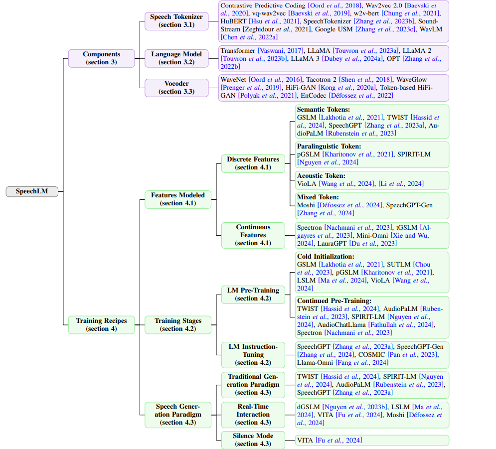
Advances in Speech Language Models (Research paper)

Components in SpeechLM

A typical SpeechLM consists of three major components, each contributing uniquely to the model’s ability to generate and understand speech.

** Speech Tokenizer**

The speech tokenizer is the first component responsible for converting continuous audio signals into latent representations. These representations are then transformed into discrete tokens or speech units, allowing the language model to process them effectively. The tokenizer’s primary objective can be divided into the following categories:

• Semantic Understanding Objective: These tokenizers focus on extracting semantic features from the audio, enabling tasks like Automatic Speech Recognition (ASR). They prioritize meaning and content over acoustic details. Popular examples include Wav2vec 2.0, W2v-BERT, and WavLM.

• Acoustic Generation Objective: These tokenizers capture the acoustic features necessary for generating high-quality speech waveforms. They are more focused on the fidelity of speech synthesis than on semantic content. Examples include SoundStream and EnCodec.

• Mixed Objective: A combination of the previous two objectives, these tokenizers balance both semantic understanding and acoustic generation. Examples include SpeechTokenizer and Mimi.

** Language Model**

The language model is at the core of SpeechLMs. These models, inspired by Large Language Models (LLMs), often utilize transformer or decoder-only architectures like OPT and LLaMA to generate speech autoregressively. They are adapted from the original text-based language models by incorporating a speech-specific tokenizer. These models are capable of handling both text and speech modalities, often expanding the vocabulary to include both types of tokens.

Token-to-Speech Synthesizer (Vocoder)

The token-to-speech synthesizer or vocoder is responsible for converting the discrete speech tokens generated by the language model back into audio waveforms. There are two main types of synthesis pipelines:

• Direct Synthesis: The vocoder directly converts speech tokens into waveforms in a straightforward, fast manner.

• Input-Enhanced Synthesis: In this pipeline, tokens are first transformed into a continuous latent representation before being fed to the vocoder. This is particularly helpful when the tokens lack detailed acoustic features, as is often the case with semantic understanding tokenizers.

The vocoder can also be chosen based on architectural preferences, such as:

• GAN-based Vocoder: Most widely used for fast and high-quality speech synthesis. Examples include HiFi-GAN and BigVGAN.

• GAN-based Neural Audio Codec: Neural audio codecs like EnCodec employ GAN architectures and are often used as vocoders in SpeechLMs.

• Other Types of Vocoder: Less common architectures include WaveNet, WaveGlow, and DiffWave, which are typically explored for specific needs in synthesis.

NLU (Natural Language Understanding) models are designed to enable computers to understand the meaning and intent behind human language, both written and spoken. These models are crucial for various applications like chatbots, voice assistants, and search engines, allowing them to process and interpret user input accurately.

cartesia

• very low latency they used State Space Models https://huggingface.co/blog/lbourdois/get-on-the-ssm-train

Vibe Voice

Step 1: Start with Understanding

• The language model (Qwen2.5) has read your text and “understands”:
  • What words should be spoken
  • Who is speaking
  • The tone and emotion
• It creates a contextual map of the speech. Think of this as a blueprint of what your audio should sound like.

Step 2: Generate Speech Tokens (Latents)

• VibeVoice doesn’t immediately make sound—it creates a compressed, abstract representation called speech latents.
• These latents capture:
  • Pitch, tone, and timbre of the voice
  • Timing and rhythm of speech
  • Speaker identity (so Alice sounds like Alice, Bob like Bob)
• The system uses diffusion models to generate these latents:
  • Start with random noise (like static on a TV)
  • Gradually refine step by step
  • After ~20 steps, you have a latent that “represents the speech perfectly”

Analogy: Imagine sculpting a statue from clay.

• Step 1: Rough blob → Step 10: recognizable shape → Step 20: polished, detailed statue.
• Diffusion is the sculpting process for sound.

Step 3: Conditioning & Guidance

• VibeVoice uses classifier-free guidance (CFG):
  • Positive condition → what you actually want to say
  • Negative condition → what you don’t want (random/unwanted sounds)
• These conditions are combined to guide the diffusion so the final audio is:
  • Clear
  • Meaningful
  • Sounds like the chosen speaker

Step 4: Decode Latents into Sound

• Once the latent vector is ready, it’s converted into a waveform using the acoustic decoder:
  • Upsamples from very low resolution (7.5 Hz) to full audio (24 kHz)
  • Preserves pitch, timbre, rhythm, and speaker characteristics
• Each chunk of speech is generated this way and stitched together for long-form audio

Analogy: The latent is like a recipe, and the decoder is the chef cooking the dish.

Step 5: Semantic Feedback Loop

• After generating a chunk, VibeVoice checks:
  • Does the audio match the meaning of the text?
  • Are the words and emotions correct?
• It uses a semantic tokenizer to encode the generated audio back into abstract features.
• These features feed into the next chunk, maintaining coherence over long speech.

Analogy: The actor listens to their own lines while performing to make sure it sounds right.

Step 6: Multi-Speaker Handling

• If multiple speakers are present:
  • Each speaker has a reference voice
  • VibeVoice generates latents for the right speaker in context
  • It ensures speaker identity stays consistent throughout the conversation

Step 7: Output

• The chunks of audio are combined into a continuous, natural-sounding audio stream.
• Even for 90 minutes of dialogue, the speech is coherent and matches the conversation flow.

https://www.tonic.ai/guides/understanding-model-memorization-in-machine-learning

https://github.com/RichmondAlake/memorizz https://modal.com/llm-almanac/summary

https://modal.com/apps/boopathi/main

piper-tts A fast, local neural text to speech system that sounds great and is optimized for the Raspberry Pi 4. Piper is used in a

• canopy

​​Speech-to-Retrieval (S2R): A new approach to voice search

check here

Other Models

• https://huggingface.co/maya-research/Veena [india hindi, english]

https://github.com/fixie-ai/ultravox

LLM inference optimization

Model compression

• Pruninig (removing unwanted wieghts)

  • Structured
  • unstructured
  • Example https://huggingface.co/neuralmagic (vllm)

• Quantization

• knowlege distillaiton

• pseudo labelling

• https://github.com/mlc-ai/mlc-llm

 Triton Server

Triton is designed to manage deep learning models in production by:
Handling concurrent requests efficiently
Managing hardware allocation dynamically
Supporting multiple frameworks like PyTorch, TensorFlow, and ONNX

LITERT

LiteRT continues the legacy of TensorFlow Lite as the trusted, high-performance runtime for on-device AI. Now with LiteRT Next, we’re expanding our vision with a new genera

https://github.com/google-ai-edge/LiteRT

MLC LLM

https://github.com/mlc-ai/mlc-llm

• https://blog.codingconfessions.com/p/groq-lpu-design

DSM

DSM is a concept used mainly in speech synthesis, speech recognition, or sequence modeling tasks (like TTS or ASR) where the system models or processes input or output sequences with a certain delay — instead of processing the entire input at once or generating output tokens immediately.

• Streaming ASR (Automatic Speech Recognition): If your recognizer waits for 100–300 ms of audio before finalizing a word, that’s DSM.
• Streaming TTS (Text-to-Speech): If your synthesizer generates audio chunks but buffers them a bit to ensure smoother prosody.
• Real-time Translation: If a system holds back a few words to get context before translating tricky word order.

Add to follow-up

Phonemes

Phonemes are the smallest units of sound in a language that can distinguish one word from another.

• Think of them as sound building blocks.
• They’re not letters—they’re sounds.

Word	Spoken Sounds (Phonemes)
cat	/k/ /æ/ /t/
bat	/b/ /æ/ /t/
Text-to-Speech (TTS) models don’t generate speech directly from letters. They first:

1. Convert text to phonemes (pronunciation),
2. Then generate audio from that.

Graphemes

Graphemes are the written characters (letters or symbols) of a language.

Word	Graphemes
“Cat”	C, A, T
“She”	S, H, E
“Phone”	P, H, O, N, E
Bytes
Bytes, in this context, refer to byte-level encodings of text—raw numerical representations of characters in a specific encoding format (usually UTF-8).

For the word “Hi”, the bytes (in UTF-8) are:

• “H” → 72
• “i” → 105

So the byte input is: [72, 105]

Byte-based models (like Bark or ByT5) bypass tokenizers and G2P (grapheme-to-phoneme) tools. They learn pronunciation from raw byte sequences.

Voice clone

• https://github.com/speechbrain/speechbrain

Voice agent testing

• Coval
• https://roark.ai/

Canary

The primary goal of the Canary project is to prove that state-of-the-art accuracy in speech recognition (ASR) and translation (AST) can be achieved without “web-scale” data

The Architectural Engine—FastConformer

To achieve this efficiency, Canary utilizes a FastConformer-based attention encoder-decoder (AED) architecture.

• The Encoder: It uses a “FastConformer” encoder, which is a speech-specific modification of a standard transformer that features an increased downsampling factor.

• The Benefit: This modification allows for a 2.8x speedup in processing without sacrificing modeling capacity.

• Prompting: Like Whisper, Canary uses special tokens to guide its tasks (e.g., <|transcribe|>, <|translate|>), but it adds new controls for punctuation and capitalization (PnC) via <|pnc|> and <|nopnc|> tokens.

Analysis: By initializing the encoder from pre-trained weights, the model converges faster and achieves better metrics than if it were trained from scratch. This architectural choice focuses on maximizing the “work” done per computation cycle.

Speech‑Augmented Language Model (SALM)?

A Speech‑Augmented Language Model (SALM) integrates speech processing with a large language model (LLM), allowing the model to understand spoken audio and text within a single framework.

The core idea is simple:

• Convert raw audio into vectors

• Make those vectors compatible with an LLM

• Let the LLM reason over audio as if it were text tokens

This bridges spoken and written language and enables multitask and in‑context learning directly in the speech domain.

2. High‑Level Architecture

SALM is a multimodal model composed of two pretrained systems joined together:

1. A Speech Encoder (from ASR models)
2. A Large Language Model (LLM)

The speech side converts sound → embeddings. The LLM side performs reasoning and generation.

3. Core Components

3.1 Audio Perception Module

This module converts raw audio into embeddings that the LLM can consume.

Subcomponents:

• Preprocessor
  Converts waveform audio into a time‑frequency representation (e.g., Mel Spectrogram).

• Encoder
  A strong ASR encoder (e.g., FastConformer from the Canary model) that extracts high‑level semantic information.

• Modality Adapter
  Adjusts encoder outputs so they align structurally with LLM expectations (often a projection or small Conformer stack).

• Projector
  A linear layer that maps audio embedding dimensions to the LLM’s embedding size.

3.2 Large Language Model (LLM)

A standard transformer‑based text model (e.g., Qwen‑2.5B) that:

• Accepts both text embeddings and audio embeddings
• Generates text output

The LLM is unchanged architecturally; only its inputs are augmented.

3.3 Tokenizer and Audio Placeholder

• Uses the LLM’s tokenizer
• Introduces a special placeholder token:

<|audio_locator|>

This token marks where audio embeddings should be inserted in the input sequence.

4. End‑to‑End Pipeline: From Sound to Vectors

We trace a 1‑second audio clip of someone saying “Cat”.

Input Audio

• Format: Raw waveform
• Sampling Rate: 16,000 Hz
• Shape:

[1, 16000]

(Batch, Samples)

5. Stage 1 — Preprocessing (Audio → Spectrogram)

Purpose

Raw waveforms are difficult for neural networks to model directly. The preprocessor converts them into a structured frequency‑time representation.

Operation

• Sliding windows (~25 ms) with ~10 ms stride
• Compute energy across Mel‑scaled frequency bins

Output

• Mel Spectrogram
• Frequency bins: 80
• Time steps: ~100

[1, 80, 100]

(Batch, Features, Time)

6. Stage 2 — Encoder (Semantic Extraction)

Model

• Canary Encoder based on FastConformer

Key Mechanisms

6.1 Temporal Subsampling

To keep sequence length manageable for the LLM:

• Time dimension is reduced by ~8× using convolutional subsampling

100 frames → ~12 frames

Each frame now represents ~80 ms of audio.

6.2 Contextual Processing

• Multiple Conformer layers combine:
  • Self‑attention (global context)
  • Convolutions (local structure)

This enables phonetic sequences to be interpreted as linguistic units.

Output Shape

[1, 1024, 12]

(Batch, Encoder_Dim, Reduced_Time)

7. Stage 3 — Projection (Audio → LLM Space)

Motivation

• Encoder output dimension ≠ LLM embedding dimension
• Alignment is required so the LLM can treat audio like text tokens

Steps

1. Transpose dimensions

[1, 1024, 12] → [1, 12, 1024]

2. Linear Projection

Linear(1024 → 4096)

Output Shape

[1, 12, 4096]

Each time step becomes an LLM‑compatible embedding.

8. What the LLM Actually Sees

Example Prompt

Transcribe: <|audio_locator|>

Embedding Construction

1. Text tokens (“Transcribe:”)

[1, 3, 4096]

2. Audio placeholder removed
3. Audio embeddings inserted

[1, 12, 4096]

Final Sequence

[1, 15, 4096]

• First tokens specify intent (what to do)
• Remaining tokens encode audio content

The LLM attends across both seamlessly.

9. Mental Model Summary

• Audio is converted into a short sequence of vectors
• These vectors are shaped to be indistinguishable from text embeddings
• The LLM reasons over intent (text) and content (audio) using the same attention mechanism

SALM does not add speech reasoning to the LLM — it reformats speech so the LLM can already reason over it.