Feature engineering

├── Data Fundamentals
│   │
│   ├── Data Types                        
│   │   ├── Tabular Data                  
│   │   ├── Image Data                    
│   │   ├── Text Data                     
│   │   ├── Time Series Data              
│   │   ├── Audio Data                    
│   │   └── Graph Data                    
│   │
│   ├── Dataset
│   │   ├── Training Set
│   │   ├── Validation Set
│   │   └── Test Set
│   │
│   ├── Features
│   │   ├── Numerical Features
│   │   ├── Categorical Features
│   │   ├── Ordinal Features              
│   │   └── Text Features                 
│   │
│   ├── Feature Engineering
│   │   ├── Feature Scaling
│   │   │   ├── Normalization (Min-Max)
│   │   │   └── Standardization (Z-Score)
│   │   ├── Encoding
│   │   │   ├── One-Hot Encoding
│   │   │   ├── Label Encoding
│   │   │   ├── Ordinal Encoding          
│   │   │   └── Target Encoding           
│   │   ├── Feature Selection
│   │   │   ├── Filter Methods            
│   │   │   ├── Wrapper Methods           
│   │   │   └── Embedded Methods          
│   │   ├── Feature Extraction            
│   │   │   ├── TF-IDF                    
│   │   │   ├── Bag of Words              
│   │   │   └── Polynomial Features       
│   │   └── Dimensionality Reduction (→ link)       
│   │
│   ├── Data Cleaning
│   │   ├── Missing Values
│   │   │   ├── Imputation (Mean/Median/Mode)       
│   │   │   └── Deletion (Listwise/Pairwise)        
│   │   ├── Outlier Detection
│   │   │   ├── IQR Method                
│   │   │   └── Z-Score Method            
│   │   ├── Data Imbalance
│   │   │   ├── Oversampling (SMOTE)      
│   │   │   ├── Undersampling             
│   │   │   └── Class Weights             
│   │   └── Duplicate Removal             
│   │
│   ├── Data Augmentation
│   │   ├── Image Augmentation            
│   │   │   ├── Flipping, Rotation, Cropping        
│   │   │   ├── Color Jittering           
│   │   │   ├── Mixup                     
│   │   │   └── CutMix                    
│   │   ├── Text Augmentation             
│   │   │   ├── Synonym Replacement       
│   │   │   ├── Back Translation          
│   │   │   └── Random Insertion/Deletion 
│   │   └── Audio Augmentation            
│   │
│   ├── Exploratory Data Analysis (EDA)   
│   │   ├── Data Visualization            
│   │   ├── Correlation Analysis          
│   │   └── Distribution Analysis         
│   │
│   └── Curse of Dimensionality           

Raw Data
│
├── Understand Data
│   │
│   ├── Variable Types
│   │   ├── Numerical
│   │   ├── Categorical
│   │   ├── Datetime
│   │   └── Mixed
│   │
│   ├── Variable Characteristics
│   │   ├── Missing Data 
│   │   ├── Cardinality               
│   │   ├── Rare Labels        
│   │   ├── Distribution   
│   │   ├── Outliers    
│   │   └── Magnitude             
│   │                             
│   └── Model Assumptions         
│                                 
├── Missing Data Handling 
│   │                                  
│   ├── Basic Imputation              
│   │   ├── Mean / Median              
│   │   ├── Frequent Category         
│   │   ├── Arbitrary Value            
│   │   ├── Missing Category           
│   │   └── Missing Indicator          
│   │
│   ├── Alternative Methods
│   │   ├── Complete Case Analysis
│   │   ├── Random Sample
│   │   ├── End of Distribution
│   │   └── Group-wise Imputation
│   │
│   └── Advanced Methods
│       ├── KNN Imputation
│       ├── MICE
│       └── missForest
│
├── Categorical Encoding 
│   │                                 
│   ├── Basic Encoding                
│   │   ├── One Hot Encoding          
│   │   ├── Ordinal Encoding          
│   │   └── Count / Frequency         
│   │
│   ├── Target-Based Encoding         
│   │   ├── Mean Encoding             
│   │   ├── Weight of Evidence        
│   │   ├── Ordered Encoding          
│   │   └── Smoothing                 
│   │
│   └── Rare Label Handling
│       ├── Group Rare Labels
│       └── Top Categories Encoding
│
├── Distribution Transformation 
│   │
│   ├── Log Transform
│   ├── Square Root
│   ├── Reciprocal
│   ├── Power Transform
│   ├── Box-Cox
│   ├── Yeo-Johnson
│   └── Arcsin
│
├── Feature Engineering
│   │
│   ├── Discretization
│   │   ├── Equal Width
│   │   ├── Equal Frequency
│   │   ├── K-Means
│   │   ├── Decision Tree
│   │   └── Binarization
│   │
│   ├── Outlier Handling 
│   │   ├── Trimming
│   │   └── Capping
│   │
│   ├── Datetime Features
│   │   ├── Date Parts
│   │   └── Cyclical Encoding
│   │
│   ├── Mixed Variables
│   │
│   └── Feature Creation
│       ├── Math Functions
│       ├── Relative Features
│       ├── Polynomial Features
│       └── Tree-Based Features
│
├── Feature Scaling 
│   ├── Standardization
│   ├── Min-Max Scaling
│   ├── Mean Normalization
│   ├── MaxAbs Scaling
│   ├── Robust Scaling
│   └── Unit Vector Scaling
│
└── Pipeline Assembly
    ├── Feature Engineering Pipeline
    ├── Classification Pipeline
    ├── Regression Pipeline
    └── Cross-Validation Pipeline

Feature selection method

Feature selection means choosing the most useful features (columns) from your dataset that best help your model make predictions.

There are five main categories of feature selection methods:

Category	Uses Statistics?	Uses Model?	Captures Interaction?	Cost
Filter	✅	❌	❌	🟢 Fast
Wrapper	❌	✅	✅	🔴 Slow
Embedded	✅	✅	✅	🟡 Balanced
Hybrid	✅ + ✅	✅	✅	🟠 Moderate
Ensemble	Multiple combined	✅	✅	🟠 Moderate

Filter Method (Statistical Base)

The Filter Method uses statistical tests between each feature and the target to measure how informative that feature is.

It filters out unhelpful features before model training.

It is called “model-independent” because it does not rely on any ML algorithm only on data statistics.

How It Works

1. For each feature Xii​:
   • Compute a statistical score showing how related Xi​ is to the target Y.
2. Rank features by their score.
3. Select the top N features or those above a threshold.

Data Type	Technique	What It Measures
Continuous–Continuous	Correlation Coefficient (Pearson, Spearman)	Linear or monotonic relationship strength
Categorical–Categorical	Chi-Square (χ²)	Independence between variables
Continuous–Categorical	ANOVA F-test	Mean differences between groups
Any type	Mutual Information (MI)	Measures shared entropy between feature and label; non-linear relationships.

Methods

• Correlation-based (for numeric features)
• Chi-Square Test (for categorical data)
• Mutual Information
• ANOVA F-Test

Limitations

• Treats each feature independently → ignores feature interactions.
• Correlation ≠ causation.
• Not tailored to a specific ML algorithm.

Example : Imagine we have features [Age, Salary, ZIP Code, Favorite Color] to predict “Loan Default”. A Chi-square or correlation test might show “Favorite Color” has no relation so you remove it before training.

Feature Type	Target Type	Method to Use
Numerical	Numerical	Pearson Correlation
Numerical	Categorical	ANOVA / Point Biserial
Categorical	Numerical	ANOVA
Categorical	Categorical	Chi-Square
Any	Any	Mutual Information

Method	What it Does	How it Works	Formula
Pearson Correlation	Measures linear relationship between numerical feature and numerical target	Calculates how much two continuous variables move together. Score ranges from -1 to +1. Near 0 means no relationship.	r = Σ(xi - x̄)(yi - ȳ) / √[Σ(xi - x̄)² × Σ(yi - ȳ)²]
Chi-Square	Measures association between categorical feature and categorical target	Compares the observed frequency of combinations vs what you’d expect if they were independent. High score = strong association.	χ² = Σ (Observed - Expected)² / Expected
ANOVA F-Test	Measures whether a numerical feature differs significantly across categorical target classes	Compares the variance between groups to the variance within groups. High F score = feature separates classes well.	F = Variance Between Groups / Variance Within Groups
Mutual Information	Measures how much a feature reduces uncertainty about the target	Comes from information theory. Calculates the reduction in entropy of the target when the feature is known. Works for linear and non-linear.	MI(X,Y) = Σ P(x,y) × log[ P(x,y) / P(x)×P(y) ]
Variance Threshold	Removes features that barely change across rows	Calculates the variance of each feature. Drops anything below a set threshold. No target needed.	Var(X) = (1/n) × Σ(xi - x̄)²
Point Biserial	Measures correlation between a numerical feature and a binary categorical target	Special case of Pearson Correlation adapted for when one variable is binary (0/1). Score ranges from -1 to +1.	rpb = (M1 - M0) / SD × √(n1×n0 / n²)
Spearman Correlation	Measures monotonic relationship between numerical feature and numerical target	Ranks both variables first, then applies Pearson on the ranks. Catches non-linear but monotonic relationships that Pearson misses.	ρ = 1 - (6 × Σd²) / n(n²-1) where d = difference in ranks
Fisher Score	Ranks features by how well they separate classes	For each feature, computes the ratio of between-class scatter to within-class scatter. Higher score = better class separation.	F = (μ1 - μ2)² / (σ1² + σ2²)

Wrapper Method (Model-Based Iteration)

Instead of statistics, the Wrapper Method uses the model’s performance to decide which features are best.

You “wrap” the selection process around the model repeatedly training and evaluating different subsets of features.

How It Works

1. Choose a base model (e.g., Logistic Regression, Decision Tree).
2. Use a search strategy:
   • Forward Selection → start with none, keep adding features that improve accuracy.
   • Backward Elimination → start with all, keep removing features that hurt accuracy.
   • RFE (Recursive Feature Elimination) → train the model, drop the least important feature each time.
3. Stop when performance no longer improves.

Forward SelectionStart empty → add bestGreedy search

What it does

Starts with zero features. At each step, tries adding every remaining feature one by one, trains a model, picks whichever feature improved accuracy the most. Repeats until adding more features stops helping.

Simple logicWorks any modelSlow on big dataMay miss combos

How it works step by step

1. Start: selected = [] (empty set)
2. Try adding each feature individually, train model, score it
3. Add the feature that gave the best score
4. Try adding each remaining feature to the current set
5. Add the next best feature
6. Stop when no addition improves score above threshold

∅→{age}→{age, salary}→stop

Simple example

Features: age, salary, height, eye colour. Target: will buy? (yes/no)

Round	Feature tried	Accuracy	Decision
1	age	72%	Add ✓
1	salary	68%	Skip
1	height	51%	Skip
2	age + salary	81%	Add ✓
2	age + height	73%	Skip
3	+ eye colour	81%	No gain → Stop

Final features kept: age, salary

Backward EliminationStart full → remove worstGreedy search

What it does

Starts with all features. At each step, removes the feature that hurts accuracy the least (i.e. the least useful one). Keeps going until removing any feature starts to hurt performance.

Sees all features firstCatches interactionsVery slow startExpensive on wide data

How it works step by step

1. Start: selected = [all features]
2. Train model with all features, record score
3. Try removing each feature one at a time, retrain, score
4. Remove the feature whose removal hurt score the least
5. Repeat — try removing each remaining feature
6. Stop when removing any feature significantly drops score

all 4→drop eye→drop height→stop

Simple example

Start with all 4 features. Accuracy with all = 81%

Round	Remove	Accuracy	Decision
1	eye colour	81%	Remove ✓ no loss
1	height	79%	Keep for now
2	height	80%	Remove ✓ tiny loss
2	salary	71%	Keep
3	age	65%	Big drop → Stop
3	salary	70%	Big drop → Stop

Embedded Method (Integrated in Model)

The Embedded Method performs feature selection while the model is being trained. It “learns” which features matter most as part of the optimization process.

How It Works

Many ML algorithms naturally assign importance to features:

• Regression coefficients
• Tree-based split importance
• Regularization penalties (L1/L2)

Embedded methods penalize complexity to shrink or zero-out unimportant feature weights.

Algorithm	Technique	How It Selects Features
Lasso Regression	L1 Regularization	Pushes some coefficients to 0 (removes features)
Ridge Regression	L2 Regularization	Shrinks coefficients (reduces importance but not 0)
Elastic Net	L1 + L2 mix	Balances both behaviors
Decision Trees / Random Forests / XGBoost	Tree-based splitting	Selects features with high information gain or Gini reduction

Hybrid Method (Two-Stage Approach)

Combine multiple methods — usually Filter + Wrapper or Filter + Embedded.

Goal: get the speed of Filter + the accuracy of Wrapper or Embedded.

Dataset Size	Feature Count	Model Type	Recommended Method
Small (< 10K samples)	Few (< 50 features)	Linear	Wrapper
Large (> 100K samples)	Many features	Any	Filter or Embedded
Medium	Moderate	Any	Hybrid
Complex / Noisy	Many features	Any	Ensemble
Sparse / High-dimensional (text, TF-IDF)	Huge (> 10K features)	Linear/SVM	Filter (Chi-square, MI)

Ensemble

Ensemble Feature Selection (EFS) borrows from ensemble learning in modeling where we combine multiple weak learners to produce a stronger, more stable model.

Similarly, EFS combines multiple feature selection outcomes to get a robust, stable, and generalizable set of features.

There are two main forms:

1. Data-Level Ensembles (Resampling-Based) We repeat the feature selection process on different data subsets and then aggregate the results.

   Example:

   1. Use bootstrapped samples of your dataset (like bagging).
   2. Apply any selection method (e.g., Mutual Information or Recursive Feature Elimination) to each sample.
   3. Count how often each feature is selected across all samples.
   4. Keep the features that are selected most frequently.

   Why this helps:

   • Random data variations are averaged out → reduces variance.
   • You get stable feature importance scores that generalize better.

2. Model-Level Ensembles (Multi-Model Based)

   We apply different models or selectors on the same dataset and aggregate their selected features.

   Example:

   • Run Logistic Regression (Embedded)
   • Run Random Forest (Embedded)
   • Run Mutual Information (Filter)
   • Combine their feature importance scores or selected feature sets.

   Aggregation strategies:

   • Voting / Ranking: Count how often a feature appears in top-K lists.
   • Weighted Averaging: Weight by model accuracy or feature importance magnitude.
   • Consensus Threshold: Select features that appear in at least X% of models.

   Why this helps:
   Different models capture different feature relationships linear, nonlinear, tree-based splits, etc. Combining them ensures generalization across model types.

Numerical Features

• Infinite Possibilities: There are endless ways to combine numerical features. Experiment with combining two, three, or more features using addition, multiplication, or other mathematical functions.
• Weighted Averages: Apply different weights to features when combining them. Normalization & Scaling: Try different scaling strategies, especially for linear models and neural networks. Experiment with Standard Scalar, Min-Max Scalar, and Max Absolute Scalar to see which performs best.
• Logarithmic Scaling: Apply a logarithm to skewed data to improve model performance.

Handling Missing Values (NaN)

• Binary Flagging: Instead of just replacing missing values with the mean, create a new binary column ( or ) indicating that the original value was missing. This informs the model that the value was imputed. Imputing with Zero: After creating the flag, replace the NaN values with zero, especially for linear models.

Categorical Features

• Target Encoding: Replace categories with the average target value for that category. Crucial: Always use a cross-validation approach to calculate these averages to prevent data leakage.
• Frequency Encoding: Replace a category with the count of how many times it appears in the dataset.
• Hashing Encoder: Use hashing to reduce the dimensionality of high-cardinality features before applying one-hot encoding, which helps manage RAM usage.
• Target Encoding Combinations: Combine multiple categorical variables into a new one, then apply target encoding to this new combined feature to capture interaction effects.

Aggregations

• Grouped Statistics: Aggregate numerical features based on categorical features. Calculate statistics like the mean, median, sum, max, min, and standard deviation for groups.

Time Series Features

• Lag Features: Create features based on past values of the target variable (e.g., target value at time t-, t-). Ensure the lag chosen allows for building features on the test set .

Advanced Techniques

• Dimension Reduction: Use PCA, LDA, SVD, or TSNE to reduce dimensionality and add these new components as features.
• Autoencoders: Use denoising autoencoders to learn compressed representations of the data and use the bottleneck layer as new features.
• Leaf Index Features: Use the final leaf indices from a trained Gradient Boosting Decision Tree (like LightGBM) as categorical features for linear models or Factorization Machines to capture complex interactions.
• Text Augmentation: For NLP, use double translation (e.g., Spanish to English to Spanish) to generate synonyms and add diversity to the training data.

Target Variable Scaling

• Log Transformation: If the target variable is highly skewed, train the model on the logarithm of the target and apply the exponential function to the predictions .

Feature Selection

• Feature Importance: Use the feature importance scores calculated by Gradient Boosting models to drop features below a certain threshold.
• Random Noise Benchmark: Add a column of random noise to the dataset. If a feature’s importance is lower than the random noise column, it is likely useless and can be dropped.
• Leave-One-Feature-Out: Pre-train a model, then evaluate the model’s performance on a validation set by shuffling or replacing one feature at a time with a fixed value (like zero or the mean) to see how much the metric drops.
• Adversarial Validation: Build a model to distinguish between training and test data to identify features that have different distributions between the two sets.

Other technique

Constant Features

A constant feature is a column where every single row has the same value.

For example, imagine a column called country and every row says India. That column tells your model absolutely nothing — there’s no variation, no signal.

Why it’s a problem if all values are the same, the model can’t learn anything from it. It’s just dead weight.

How to find them — you check if the number of unique values in a column is exactly 1. In pandas you’d use nunique() and drop any column where the result is 1.

Quasi-Constant Features

These are columns where one value appears in 99% (or more) of the rows, and the rest of the values are rare exceptions.

For example, a column called has_profile_photo where 99.5% of users have a photo. The column is technically not constant, but it’s close to useless because there’s barely any variation.

Why it’s a problem the model sees almost the same value everywhere, so it can’t use the column to distinguish between outcomes reliably.

How to find them —you calculate what fraction of rows the most common value occupies. If it’s above a threshold like 0.99 or 0.995, you drop it.

The threshold is your choice depending on the problem. 0.99 is a common starting point.

Duplicated Features

These are columns that contain exactly the same values as another column, just possibly with a different name.

For example, income_usd and salary_usd might both hold the exact same numbers. Or sometimes during data pipelines, the same column gets added twice by mistake.

Why it’s a problem — having two identical columns doesn’t give your model more information. It just increases dimensionality and can cause issues with models that are sensitive to correlated inputs.

How to find them — you transpose your dataframe and find duplicate rows (which correspond to duplicate columns in the original). In pandas, df.T.duplicated() does exactly this.

Correlated Features

Two features are correlated when they carry very similar information, even if they’re not identical.

For example, height_cm and height_inches — obviously the same thing in different units. Or age and years_of_experience — not identical, but they tend to move together closely.

Why it’s a problem — it creates redundancy. The model ends up learning from the same signal twice, which doesn’t help and can destabilize some models like linear regression.

How to find them — you build a correlation matrix and look for pairs of features with a correlation above a threshold like 0.9 or 0.95. Then you drop one from each pair.

normalizing training sets

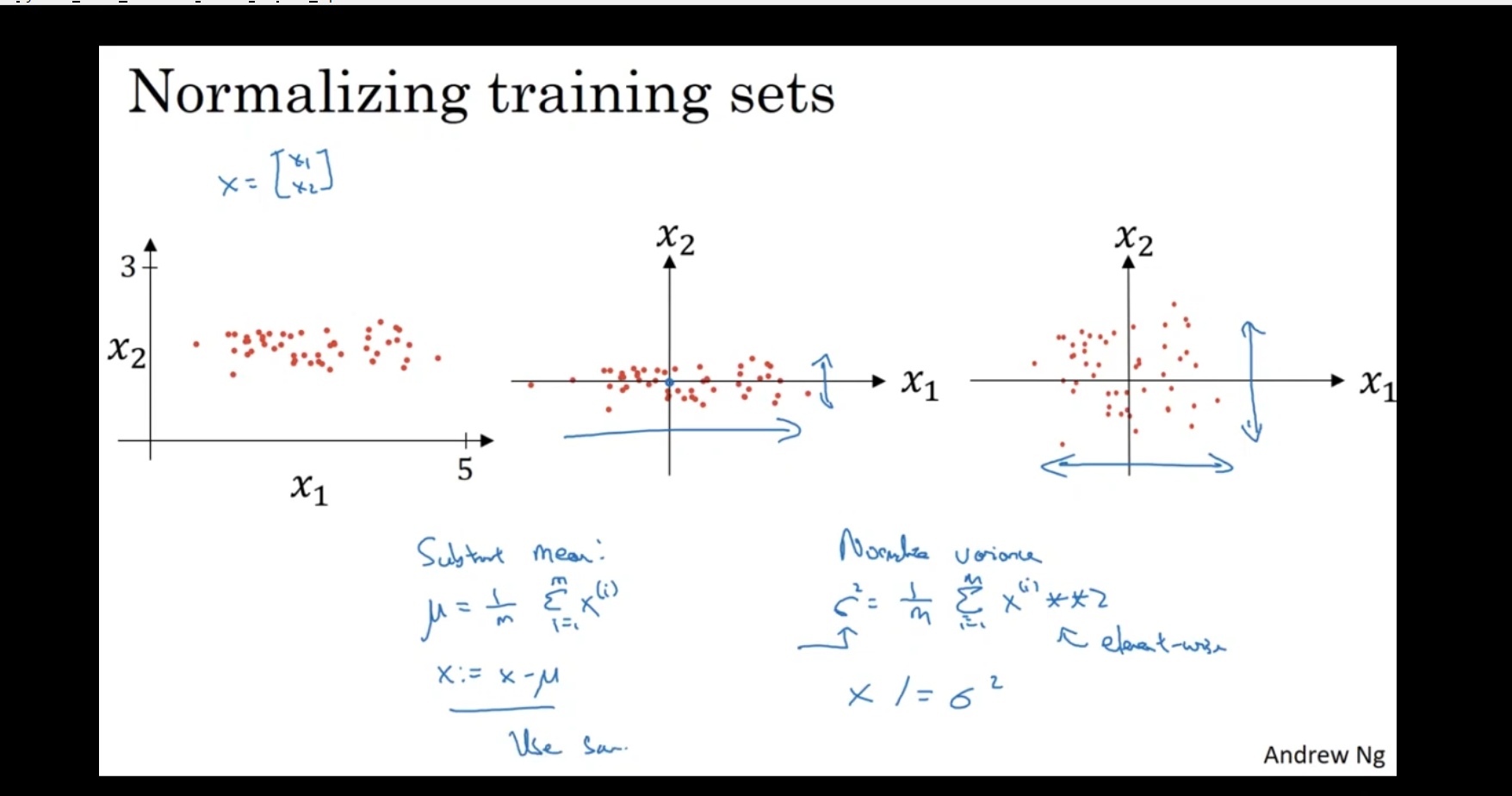
Feature Normalization:

The image shows two features ($x_1$ and $x_2$) and how normalization of features can be done before training a machine learning model.

2. Data in the Image:

• The left part shows data where the feature $x_1$ has a much larger range than $x_2$. Here, $x_1$ spans from 0 to 5, while $x_2$ has a smaller range (e.g., 1 to 3).
• The goal is to normalize this data, so both features have similar scales, which helps algorithms like gradient descent converge faster.

2. Subtraction of Mean:

• Mean Subtraction: The blue text on the bottom left indicates the calculation for normalizing the data by subtracting the mean:

$$\mu =\frac{1}{m}\sum _{i=1}^m{x}^{(i)}$$

where $m$ is the number of data points, and $x^{(i)}$ is the value of feature $x$ for the $i$-th data point.

• By subtracting the mean $\mu$, we center the data around 0. This helps make the training more stable.

Normalizing the Variance:

• Variance Normalization: The blue text on the bottom right indicates the formula for normalizing the variance (standardization):

$$x^{\prime }=\frac{x-\mu }{\sigma }$$

where $\sigma$ is the standard deviation of the feature, and $x^{\prime }$ is the normalized feature. This scales the data to have a mean of 0 and a variance of 1.

• By normalizing both the mean and the variance, each feature will have a similar scale, making it easier for algorithms to process the data effectively.

Visualizing Normalization:

• After normalization, the data will be spread out more evenly along the axes of $x_1$ and $x_2$, making the dataset more balanced in terms of the features’ ranges.

Why Normalize Data?

• Improves convergence in gradient descent: When features have very different scales, gradient descent might take longer to converge. Normalization helps in faster convergence by giving each feature equal importance.

• Prevents bias: Without normalization, features with larger values (e.g., $x_1$) could dominate the model’s learning process. Normalizing ensures that each feature contributes equally.

• Improves performance: Some algorithms (like SVMs, K-means, and neural networks) assume that the data is normalized or standardized. This ensures that the algorithm performs better.

Methods of Normalization:

• Standardization (Z-score normalization): Subtract the mean and divide by the standard deviation for each feature.
• Min-Max Scaling: Scale the data to a fixed range, usually [0, 1].

Normalization is especially important for models like SVMs, k-NN, and neural networks where the scale of the input features affects model performance.

Hashing

Feature hashing, or the hashing trick, is a machine learning technique that converts high-dimensional, categorical data into a fixed-size numerical vector by using a hash function.

How it works

1. Hashing:  A hash function is applied to each categorical feature (e.g., a word or a user ID). 

2. Indexing:  The hash function outputs an integer, which is used as an index in a pre-defined, fixed-size vector. 

3. Updating:  The value at that index in the vector is updated based on the feature. A signed hash function is often used to help mitigate collisions and preserve some information. 

4. Vector Creation:  The resulting fixed-size vector is then used as input for the machine learning model.

Python package

• https://feature-engine.trainindata.com/en/latest/