
Regression Losses
Mean Bias Error (MBE) – Captures average bias in predictions. Rarely used since positive and negative errors cancel out.
Mean Absolute Error (MAE) – Average absolute difference between predicted and actual values. Treats small and large errors equally since gradient magnitude is constant.
Mean Squared Error (MSE) – Squares errors, making large errors count more. Useful, but sensitive to outliers.
Root Mean Squared Error (RMSE) – Square root of MSE. Keeps loss in the same units as the target variable.
Huber Loss – Hybrid of MAE and MSE. Acts like MSE for small errors and MAE for large ones. Needs a hyperparameter to define the transition point.
Log-Cosh Loss – Smooth, non-parametric alternative to Huber. More stable but a bit more computationally expensive.
Classification Losses
Binary Cross-Entropy (BCE) – Standard for binary classification. Measures mismatch between predicted probabilities and true labels.
Alright — let’s rebuild Binary Cross-Entropy (BCE) from the ground up, like you were discovering it for the first time.
We want the model to output a probability ( p in [0,1] ) — not just a hard 0 or 1 — because we want to measure how confident it is.
Now, we need a loss function that tells us:
“How bad is the model’s predicted probability ( p ) compared to the true answer ( y )?”
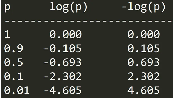
We take negative of log(p) just to make it positive. If the model is confident and correct (p ≈ 1), -log(p)≈ 0. If it’s wrong and gives a small probability to the true class (p ≈ 0), the loss shoots up.
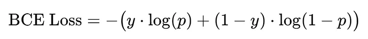
As we said, we have two classes (1 and 0).
If the true label is 1, then only the first term matters: −log(p) and the second term becomes zero. So, the loss punishes low p values, the model must make p → 1.
If the true label is **0 **, then only the second term matters: −log(1−p) and the first term disappears. Now, the loss punishes high p values, the model must make p → 0.
We add both terms because we don’t know in advance whether the label will be 0 or 1. It is just a smart way to combine both cases into one single equation. Depending on whether y=1 or y=0, one term automatically becomes active, and the other goes to zero.
| True label ( y ) | Predicted ( p ) | Desired penalty |
|---|---|---|
| 1 | 1.0 | 0 (perfect) |
| 1 | 0.9 | small |
| 1 | 0.1 | huge |
| 0 | 0.0 | 0 (perfect) |
| 0 | 0.1 | small |
| 0 | 0.9 | huge |
Example
| y | p | -[y log(p) + (1-y) log(1-p)] | Meaning |
|---|---|---|---|
| 1 | 0.9 | 0.105 | good (low loss) |
| 1 | 0.5 | 0.693 | uncertain (medium loss) |
| 1 | 0.1 | 2.302 | bad (high loss) |
| 0 | 0.1 | 0.105 | good (low loss) |
| 0 | 0.5 | 0.693 | uncertain (medium loss) |
| 0 | 0.9 | 2.302 | bad (high loss) |
Because:
- If y=1 the second term vanishes →
- If y=0: the first term vanishes →
Hinge Loss – Based on the margin between points and decision boundary. Penalizes wrong predictions and low-confidence correct ones. Used in training SVMs.
Cross-Entropy Loss
Binary Cross Entropy worked great when we had only two classes.
Now it’s multi-class classification and here comes Cross Entropy Loss. When we have more than two classes, the model doesn’t just give us one probability. Instead, it gives a probability distribution over all classes.
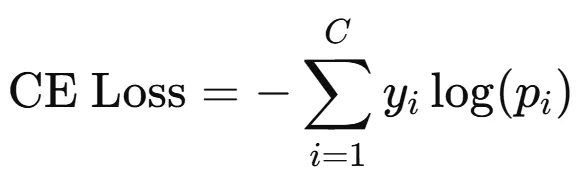
After training with Cross Entropy Loss, the model learns to assign high probability to the correct class and very low probabilities to all other classes. In other words, for a given input, the output probability distribution becomes sharp and confident, with the true class close to 1 and the rest close to 0. This is the result of the model learning from the loss function over many examples.
Balanced Cross Entropy
KL Divergence – Measures how one probability distribution diverges from another. For classification, minimizing KL is equivalent to minimizing cross-entropy, but it’s widely used in t-SNE and knowledge distillation.