Optimization and Hyperparameter in ML

├── Optimization
│   ├── Objective Function
│   ├── Convex Optimization
│   ├── Non-Convex Optimization     
│   ├── Constrained Optimization    
│   │   └── Lagrange Multipliers    
│   ├── Gradient Descent
│   │   ├── Batch Gradient Descent
│   │   ├── Stochastic Gradient Descent
│   │   └── Mini-Batch Gradient Descent
│   ├── Momentum
│   ├── Nesterov Momentum
│   ├── RMSProp
│   ├── Adam
│   ├── Adagrad
│   ├── AdamW
│   ├── LAMB                        
│   ├── Learning Rate Scheduling    
│   │   ├── Step Decay              
│   │   ├── Exponential Decay       
│   │   ├── Cosine Annealing        
│   │   ├── Warmup                  
│   │   ├── Cyclic Learning Rate    
│   │   └── ReduceLROnPlateau       
│   ├── Gradient Clipping           
│   └── Second-Order Methods        
│       ├── Newton's Method         
│       └── L-BFGS 

we have data points:

$$(x_i,y_i)$$

we assume a model:

$$\hat{y}=wx+b$$

This is not “the answer”it’s just a function with adjustable parameters (w, b).

So the real question becomes:

Which values of (w) and (b) make this function match the data best?

We need a numerical score that tells us how bad the model is.

So we define a cost function:

$$J(w,b)=\frac{1}{N}\sum _{i=1}^N(w{x}_i+b-y_i{)}^2$$

Break it down mechanistically:

• (wx_i + b) → model prediction
• (y_i) → actual value
• difference → error
• square → penalize large errors more
• average → single number

So:

The cost function converts “how wrong the model is” into a single scalar value.

Optimization = finding (w, b) that minimize (J(w, b))

“search in parameter space for minimum error”

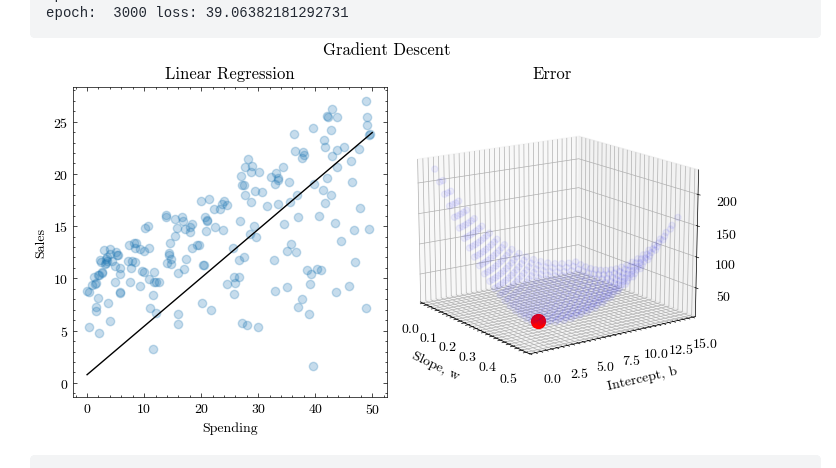
First graph (data space)

• x-axis → input (Spending)
• y-axis → output (Sales)
• line → model

This shows:

What the model does

Second graph (parameter space)

• axes → (w) (slope), (b) (intercept)
• height → (J(w, b)) (error)

This shows:

How good each possible model is

we are not optimizing in data space.

we are optimizing in parameter space:

• each point = one model
• height = its error

So:

The surface is a map: “If we choose this (w, b), your error will be this much”

How do we move toward the minimum?

We need:

• direction to move
• step size

This comes from gradients.

Gradient = local slope of error surface

Gradient = vector of partial derivatives

$$\nabla f=\left[\begin{array}{c}\frac{\partial f}{\partial x}\frac{\partial f}{\partial y}\end{array}\right]$$

Let:

$$f(x,y)=x^2+y^2$$

Step 1: differentiate

$$\frac{\partial f}{\partial x}=2x$$ $$\frac{\partial f}{\partial y}=2y$$

Step 2: form gradient

$$\nabla f=\left[\begin{array}{c}2x2y\end{array}\right]$$

At point (1, 2):

$$\nabla f=\left[\begin{array}{c}24\end{array}\right]$$ $$\frac{\partial J}{\partial w},\frac{\partial J}{\partial b}$$

These tell:

• If we increase (w), does error go up or down?
• If we increase (b), does error go up or down?

Update rule

$$w:=w-\eta \frac{\partial J}{\partial w}$$ $$b:=b-\eta \frac{\partial J}{\partial b}$$

Where:

• (\eta) = learning rate

Why subtraction?

Because gradient points in direction of increase. We want decrease, so we go opposite.

Stochastic Gradient Descent

Adam optimization

Adaptive moment estimation

Hyperparameter

$\alpha$ (Learning Rate)

The learning rate determines the size of the steps the optimizer takes during training to minimize the loss function.

• If the learning rate is too high, the model may overshoot the optimal point.
• If the learning rate is too low, the training may be slow and may get stuck in local minima.
• Choosing the right $\alpha$ is crucial for model convergence.

${\beta }_1$ and ${\beta }_2$ (Momentum Terms)

These are the decay rates for the first moment (${\beta }_1$) and the second moment (${\beta }_2$) used in the Adam optimizer.

• ${\beta }_1$ controls the moving average of the past gradients (momentum).

• ${\beta }_2$ controls the moving average of the past squared gradients (used to scale the learning rate for each parameter).

• ${\beta }_1$ close to 1 (like 0.9) gives more weight to past gradients, helping to smooth updates.

• ${\beta }_2$ close to 1 (like 0.999) makes the updates smoother by considering larger variations in the gradients.

$ϵ$ (Small Constant for Numerical Stability)

A small value (like $10^{-8}$) added to the denominator in optimization algorithms (like Adam) to avoid division by zero when the denominator becomes too small.

• Effect: It helps stabilize computations, particularly when the moving averages become very small.

layers (Number of Layers in the Model)

This refers to the total number of layers (such as input, hidden, and output layers) in a neural network.

• More layers allow the model to learn more complex patterns, but it also increases computational complexity and the risk of overfitting.
• Deep networks with many layers can capture more intricate relationships in data but require more careful training.

hidden units (Number of Hidden Units per Layer)

This defines the number of neurons in each hidden layer of the neural network.

• More hidden units can allow the network to learn more complex representations of the data.
• However, increasing the number of hidden units may lead to overfitting and higher computational costs.

Learning Rate Decay

The learning rate decay refers to reducing the learning rate as training progresses.

• This can help the model converge more smoothly. When the model is close to an optimal solution, a lower learning rate ensures more precise updates.
• Learning rate decay can be implemented in various ways, such as exponential decay or step decay, where the learning rate decreases at fixed intervals.

Mini-batch Size

The mini-batch size refers to the number of training examples used in one iteration of training.

• Smaller mini-batches tend to provide more frequent updates, which can make the training process faster but also noisier.
• Larger mini-batches provide more stable estimates of the gradient but may require more memory and computational power.
• Trade-off: A good choice of mini-batch size balances the stability of training and computational efficiency.

Resources

• Gradient descent made better Vizuara