
├── Linear Algebra
│   ├── Scalars
│   ├── Vectors
│   │   ├── Vector Addition
│   │   ├── Vector Norms
│   │   │   ├── L1 Norm
│   │   │   ├── L2 Norm
│   │   │   └── Max Norm (L∞)
│   │   ├── Dot Product
│   │   ├── Cross Product
│   │   ├── Cosine Similarity
│   │   ├── Orthogonality
│   │   └── Projection
│   │
│   ├── Matrices
│   │   ├── Matrix Addition
│   │   ├── Matrix Multiplication
│   │   ├── Transpose
│   │   ├── Inverse
│   │   ├── Determinant
│   │   ├── Trace
│   │   ├── Matrix Norms (Frobenius, Spectral)
│   │   ├── Symmetric Matrices
│   │   ├── Positive Definite Matrices
│   │   ├── Orthogonal Matrices
│   │   └── Sparse Matrices
│   │
│   ├── Tensors
│   │   ├── Tensor Operations
│   │   └── Tensor Decomposition
│   │
│   ├── Linear Transformations
│   ├── Span and Linear Independence
│   ├── Basis and Dimension
│   ├── Eigenvalues
│   ├── Eigenvectors
│   ├── Diagonalization
│   ├── Singular Value Decomposition (SVD)
│   ├── Rank
│   └── Pseudoinverse (Moore-Penrose)
Straight line
The slope tells us how many units we move vertically (up or down) for every unit we move horizontally (right or left).
y = mx+b
m = x2-x1/y2-y1
Vector
A vector is more than just an arrow on a graph. It’s a container of information it can hold direction, position, or a list of attributes describing a real-world object.
Imagine you’re evaluating houses. Each house has:
- Floor area (in sq. ft)
- Number of bedrooms
- Number of bathrooms
- Price (in thousands)
You can represent a house as a vector:
h = [
		1800
		30
		2
		230
	]
Now, all houses in your dataset become points in 4D space, where each axis is an attribute. This way, you can compare houses geometrically e.g., how “far apart” they are in feature space.
In physics, a vector might represent:
- Velocity: 30 m/s north
- Force: 100 N at 45°
So vectors aren’t just lists they mean something. A force vector tells you how hard and in which direction something is being pushed.
Vector concepts
Vector length (norm / magnitude)
Euclidean distance from origin to the vector’s tip
If a vector is →v = (3, 4), then draw it from the origin to the point (3, 4).
That forms a right triangle with sides 3 and 4.
The formula for distance between two points was
For our case x2 and y2 are 0 because it is in origin so
Norm vector
A normal vector (or norm vector) is a vector that is perpendicular to a given surface, line, or plane.
In the context of 2D geometry, for a line in the form , the normal vector is a vector that points perpendicular to the line. This vector is defined by the coefficients of and in the line’s equation.
For the line :
Same the equation of line represent in slope form is y = mx+b
The normal vector is:
Why is it called a “normal” vector?
- The word “normal” comes from the mathematical term “normal to,” meaning “perpendicular.”
- A normal vector is perpendicular to the line (or plane, in 3D) it is associated with.
How is it used?
The normal vector tells you the direction of the line’s “steepness” or “slope” and is essential for various calculations, such as:
- Finding the shortest distance from a point to a line
- Defining the orientation of the line.
Consider the line :
- The normal vector is .
- This vector is perpendicular to the line at every point, and it provides the direction you would travel to get from the line in a straight path.
How to find Normal vector?
Let’s say you have a point that lies on the line. For this point to satisfy the equation of the line, when you plug and into the equation, it must result in 0:
This means that the point satisfies the line’s equation.
Vectors and Dot Product:
Now, let’s think about this in terms of vectors.
Position Vector of the Point:
The position vector of the point is simply the vector from the origin to the point. This is written as:
Normal Vector:
Now, the normal vector to the line is defined as , where and are the coefficients from the line’s equation. The normal vector is always perpendicular to the line, which means that it points in the direction that is orthogonal (at a 90° angle) to any vector lying on the line.
Why the Dot Product is Zero: The dot product of two vectors and is given by:
Here’s the key idea:
- For two vectors to be perpendicular, their dot product must be zero. This is because the dot product measures how much one vector “projects” onto the other. If the vectors are perpendicular, there’s no projection, so the dot product is zero.
In our case:
-
If the point lies on the line, then the equation is satisfied.
-
This implies that the dot product equals .
-
So the dot product gives you a measure of the distance from the origin to the point, but it doesn’t affect the fact that the vector is perpendicular to any vector along the line.
Thus, is normal to the line because the dot product of the normal vector with any vector lying along the line will always be zero.
Dot product
A scalar value that tells us how much one vector goes in the direction of another
How much of vector w⃗ lies in the direction of v?
Depending on the sign of the result:
- Positive → Vectors point roughly in the same direction
- Zero → Vectors are perpendicular (orthogonal)
- Negative → Vectors point in opposite directions
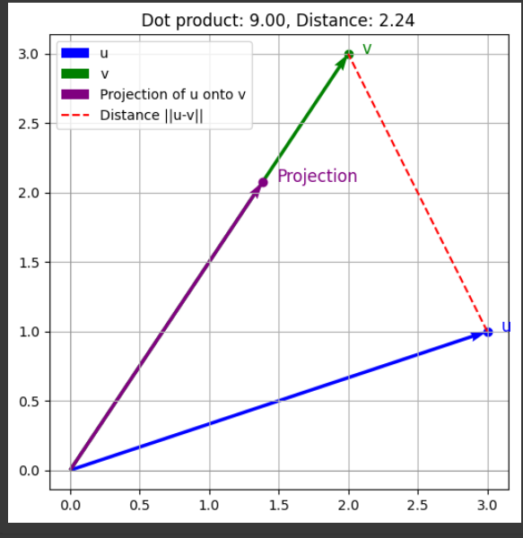
- Blue vector = u, Green vector = v.
- The red dashed line is the actual distance ∥u−v∥ between them.
- The dot product u⋅vu \cdot vu⋅v is not this red length. Instead, it measures how much u “falls” in the direction of v(a projection).
Example
Imagine we trying to predict whether a movie will be liked by a user based on the user’s preferences (represented by a vector) and the movie’s attributes (e.g., genre, director, actors, etc., also represented as a vector). The dot product between the user’s preference vector and the movie’s feature vector can tell you how much the movie “aligns” with the user’s preferences. If the dot product is large, the movie is likely to be liked; if it’s small or negative, the movie is less likely to be liked.
- Movie vector: (representing Action genre, Christopher Nolan, Tom Hardy)
- User vector: (representing moderate Action interest, love for Nolan, dislike of Tom Hardy)
- Dot product: 166 (tells us how well this movie matches the user’s preferences).
To get the threshold like if dot product above 150 user like etc.
calculate the threshold based on historical data. The idea is to set the threshold so that it accurately predicts whether users will like or dislike a movie based on their past behavior
Angle between two vectors
Introduced via the cosine formula in the dot product
Projection of one vector onto another
The component of one vector that “falls” onto the line of the other
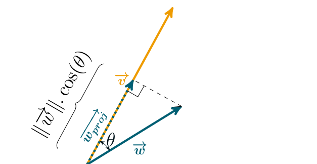
- “How much of A points in the direction of B?”
- Its length is how much A “lies along” B.
- The difference between A and its projection is perpendicular to B.
Linear Combination
A linear combination means we’re creating new vectors by scaling and adding existing ones.
we have unit vector which can be represent all other vector
Assume we have two number 2 and 3 that is alpha and beta if we muliptly we get a vector
Linearly independent
-
Linearly independent vectors are like arrows pointing in different directions, so none of them can be created by stretching or combining the others.
-
If you cannot write one vector as a combination (stretching + adding) of the others, then those vectors are linearly independent.
-
Vectors are linearly dependent if at least one vector can be made by stretching and adding the others.
we can represent the z vector by w vector if we multiply w by 2
Note: If vector is linearly dependent mean there is reduncey in vector we can remove unwanted vector.
Span
The span of vectors is the set of all possible linear combinations of those vectors.
Span is nothing but we can create any no of vector by replacing the alpha and beta in our linear combination that what span
if we multiple by our scaler alpha and beta of i and j we get new vector if keep changeing the alpha and beta we get new points
We can multiply any number we get points if we map all points in graph we can represent anywhere in the map
minimal spanning set is:
- A spanning set with no unnecessary (redundant) vectors.
- You already can reach all points in the space without it.
- It’s not giving you any new direction.
- Example {(1,0),(0,1),(1,1)}
- This means (1,1) is a linear combination of the other two.
- If you remove (1,1), you still have the full plane → the span is unchanged.
- ❌ Redundant vector → Not minimal.
- So this is not basis
- If you remove any vector from it, it no longer spans the space.
In other words: You keep the set as small as possible while still covering the whole space.
basis
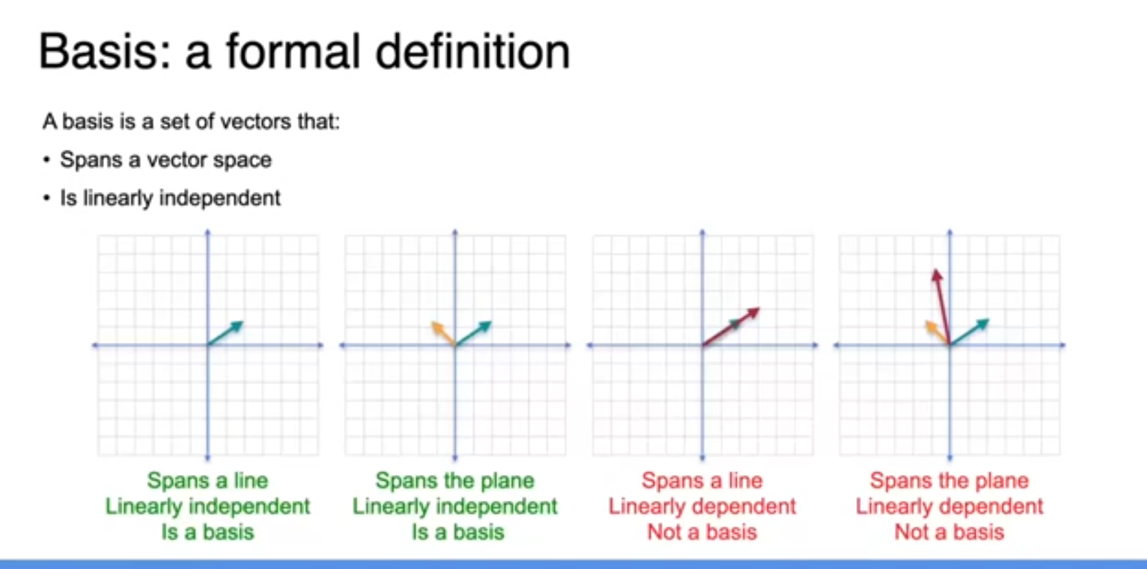 A basis is a minimal set of independent vectors that can span a space. our bias for 2D
Let take example we have vector of data for rooms so we have vector for no of bedroom and bathroom represent as
x - 2y = 0
2x - 4y = 0


second example where they not crossed over origin
x - 2y = 3
2x - 4y = 6
If we plot that in graph we get two same line both are linearly dependent
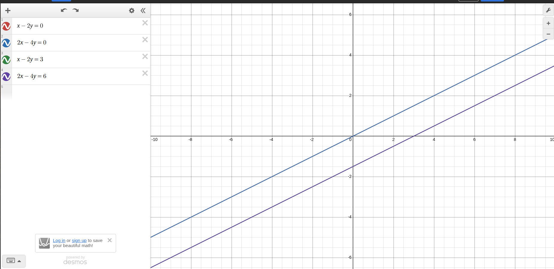
If we solve the equation
x= 2y
so if we take what every x y is double then x that what it trying to say so the biasis for this 2,1
A basis vector like 2,1 is the smallest, simplest arrow that points exactly along the solution line.
We can able to plot all the data points in line by using 2,1
Every other solution is just that arrow, stretched or flipped.
Basis and Coordinate Systems
Vector basis
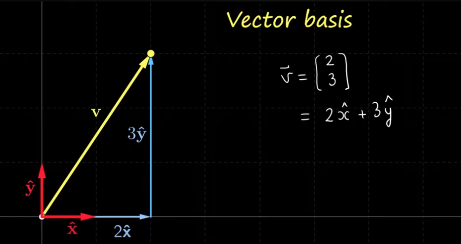
Assume we have unit vector of 1 unit of x Axis and Y axis if we multiple the unit vector with 2 and 3 we get our vector v
So every vector we can represent by using unit vector which is called vector basis
We have choosed the x1 and y1 as basis but we can choose any basis as base for vector
Vector vs Matrix
-
A vector can represent a single data point with multiple features (or dimensions). For example, a vector represents one data point with nnn features.
-
A matrix can represent multiple data points, each having multiple features. For example, an m×nm \times nm×n matrix represents mmm data points (rows), each with nnn features (columns).
A matrix is a rectangular arrangement of numbers, symbols, or functions organized in rows and columns. Its size (or order) is given by the number of rows m and columns n. We denote this as:
For example, a 3×3 matrix looks like this:
More generally, a matrix can be represented as:
Matrices in Machine Learning
In machine learning, matrices are often used to organize features measurable properties or characteristics of the data for multiple samples.
Suppose we want to predict whether students will make the basketball team based on three features:
- Height (in meters)
- Weight (in kilograms)
- Average grade (on some scale)
Each student is represented as a vector of features:
Combining all students’ vectors forms a feature matrix XX:
Alongside this matrix, you might have a target vector yy indicating if each student made the team:
This dataset (feature matrix + target vector) is then used to train machine learning models.
Matrices Linear Transformations
Matrices are machines that act on vectors to transform them. They rotate, scale, flip, or skew the vector space.
Example : When we apply a filter, it alters the brightness, contrast, and color tones.
What’s happening under the hood? The pixels are vectors of RGB values, and the filter is a matrix transformation:
Linear Transformation
A linear transformation is a rule (or function) that takes a vector as input and gives another vector as output in a way that preserves straight lines and scales/proportions.
But need stasify these rules
- Additivity: T(u+v)=T(u)+T(v)
- Homogeneity:T(c⋅v)=c⋅T(v)
What does a linear transformation look like?
- Stretching
- Rotating
- Reflecting
- Shearing (slanting)
- Compressing
- Identity (does nothing)
But no:
- Bending curves
- Shifting (translation)
- Warping
Determinant
Is the area between two vector reprsent as in matrix
a b
c d
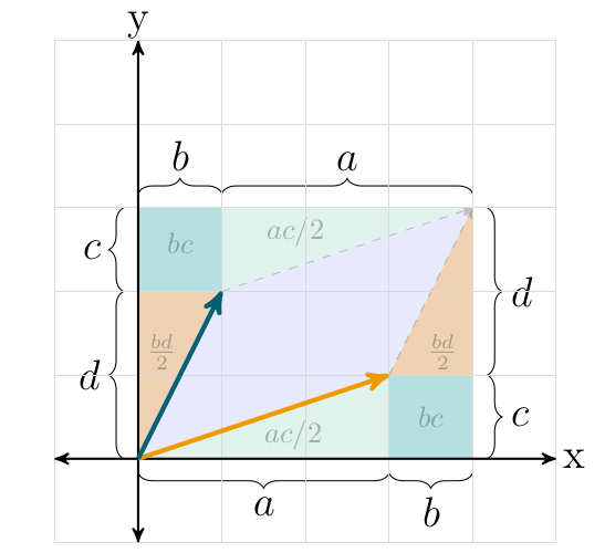
How the formula came
(a + b)(c + d) − ac − bd − 2bc = ad − bc
Let’s take:
- v₁ = (2, 1)
- v₂ = (3, 4)
Then:
Area=∣2×4−1×3∣= ∣8−3∣ =5
That means these two vectors span a parallelogram with area 5.
We can compute area before and after linear transformation and it tell
- Determinant = 1 → area stays the same
- Determinant = 2 → area doubles
- Determinant = 0 → area is 0 → the transformation collapsed everything into a line (no area) also they are linearly dependent vector
Column space
The only building blocks for outputs are the columns of the matrix.
Columns:
If we feed in (x,y) to A
So every output is some combination of these two columns.
That’s the column space:
- All vectors you can make by combining the columns.
- If c1 and c2 are independent → column space is a plane in
- If they are dependent (one is multiple of the other) → column space is a line in
Rank
The number of independent columns (or rows it’s the same).
- Rank = dimension of the column space.
- Rank tells you how many independent directions the matrix can produce.
Rank tell how it look in graph does it was 2D or 3D etc
let say if we have matrix
1 2
2 3
IF we multiply by any vector x,y we able to cover all space in 2D plane because both are linearly independent so the RANK is 2
1 2
3 6
Here they are linearly dependent where they have only line if multiply by any vector it will be on line only
Methods to find rank
There are 3 common ways:
- Row-reduction (Gaussian elimination) → Most practical by hand.
- Determinants → Works for square matrices (check minors).
- Singular Value Decomposition (SVD) → Used in computers.
The application of RANK help us to reduce the size of image let say we have image with matrix 264*264 l
The rank of a matrix tells you how many independent rows (or columns) it has.
- If rank = no of rows, all rows/columns are independent → you need all of them to represent the data exactly.
- If rank is smaller, the rest of the rows/columns can be expressed as combinations of a few independent ones.
If most of an image’s matrix can be reconstructed from a few independent components, we can store only those and throw away the rest reducing size.
If one row is exactly the average of two other rows, we don’t need to store it — we can just say:
If one row is exactly the average of two other rows, we don’t need to store it — we can just say:
Null space and kernel
A linear transformation of a matrix take in to the zero of the origin If you have a matrix A and you solve:
Any solution X you find is a null space vector.
Those vectors are special because:
- They get completely erased by the transformation A they become the zero vector.
- Geometrically, they’re the directions that get squashed to a single point at the origin.
If we mulitply (linear transformation) by vector which give us zero which is called null or kernel vector
Null space
If we multiply a matrix by any vector it will always give 0
Invertablity
A matrix is invertible if we can “undo” the transformation it performs.
Just like how the inverse of a number “undoes” its multiplication:
5 * 1/5 = 1
For a matrix A, if there exists another matrix
where I is the identity matrix), then A is invertible.
- If det(A)≠0, then the matrix is invertible.
- If det(A)=0, then the matrix is not invertible.
| Matrix | Effect | Determinant | Sign Meaning |
|---|---|---|---|
| Scaling only | Expands or shrinks space | >0 | Preserves orientation |
| Rotation | Just rotates space | >0 | Preserves orientation |
| Reflection | Flips like a mirror | <0 | Reverses orientation |
| Degenerate | Squashes space (flat) | =0 | Loses dimension |
A matrix has an inverse only if:
- It is square (same number of rows and columns), and
- Its determinant is not zero
systems of linear equations
A system of linear equations is just a way to express relationships like:
We want to find the values of x and y that satisfy both equations at the same time.
A- the coefficient matrix
we can now use matrix techniques (like inverse matrices) to solve the system all at once.
This means we just compute the inverse of A, multiply by b⃗ and we get your solution
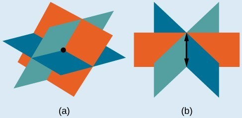
- Homogeneous: Geometrically, solutions form a subspace (passes through the origin). Ax=0
-2x+y−3z=0−x+4y+z=0

 Homogeneous equations always have at least one solution the trivial solution
x=0,y=0,z=0
- Non-homogeneous: Solutions form an affine space (shifted, does not necessarily pass through origin). Ax=b
2x+y−3z=5−x+4y+z=−2
Eigenvectors
Imagine we apply a transformation (matrix) to a vector. Most vectors change direction and length.
But some very special vectors only change length, not direction.
Those are called eigenvectors.
And the amount they stretch/shrink by is called the eigenvalue.
If we multiply a matric by a vector v we get some output but we can take the common scale from the output which again give our vector
Example
M  = 2 1
	 1 2

vector = 1
		 1

if we multiply M * v =  3
						3

But if we take 3 outside we again get the vector v 3 = 1
														1


so the eigenvector is 1,1 and eigenvalue is 3

That what telling in formula
	A * v = lambda * vector -> which eignvector and vaule
Av=λv
Where:
- A is the transformation matrix,
- v is the eigenvector (must be non-zero),
- λ is the eigenvalue (a scalar).
It means:
“When we apply A to v⃗, we just scale it by λ— no rotation.”
If we solve the equation we get formula to find eigenvaules and vector
Av−λv=0

Factor out v

(A−λI)v=0

We now want non-zero v⃗ to satisfy this, which is only possible if:

det(A−λI)=0

This gives us a characteristic polynomial in λ, whose roots are the eigenvalues.
Indepth
Eigenvectors make understanding linear transformations easy. They are the ‘axes’ (directions) along which a linear transformation acts simply by ‘stretching/compressing’ and/or ‘flipping’; eigenvalues give you the factors by which this compression occurs.
Matrix Diagonalization
Matrix Diagonalization is the process of rewriting a matrix in a simpler, diagonal form using its eigenvectors and eigenvalues.
Matrix diagonalization is the process of expressing a matrix A as:
A=PDP^−1
- D is a diagonal matrix with the eigenvalues of A on the diagonal.
- P is a matrix with the eigenvectors of A as its columns.
Diagonalization is like changing the basis of a matrix so it becomes simpler (diagonal), allowing:
- Easy computation of powers
- Insight into matrix structure
- Application to physics, ML, control systems
To find eigenvalues by solving the characteristic equation:
det(A−λI)=0
- Detereminted * a - lambda * I = 0
Orthogonal
Two vectors are orthogonal if their dot product is zero:
This means they’re perpendicular and independent.
A vector is normal (in this context) if its length is exactly 1:
This is called a unit vector — it keeps only the direction, not extra size.
A set of vectors is orthonormal if:
- Orthogonal to each other
- Normal (unit length) individually
So:
- Orthogonal = perpendicular, but can be any length.
- Orthonormal = perpendicular and each one is length 1.
Orthogonal but not orthonormal:
Dot product is , but lengths are and . Orthonormal version (divide each by its length):
Dot product is still , but now lengths are .
Matrix Decomposition
Matrix Decomposition (or Factorization) means expressing a matrix as a product of simpler matrices that are easier to analyze or compute with.
- break a number like 606060 into 2×2×3×52
- break a function like sin(x)\sin(x)sin(x) into a Taylor series
- break a sound into frequencies (via Fourier transform)
| Name | Works On | Purpose |
|---|---|---|
| LU Decomposition | Square matrices | Efficiently solve linear systems Ax=bAx = b |
| QR Decomposition | Any matrix | Used in least squares, numerical stability |
| Cholesky Decomposition | Symmetric, pos-def | Faster version of LU for specific matrices |
| Eigen Decomposition | Square matrices | Diagonalize matrices (if possible) |
| SVD (Singular Value) | All matrices (any size) | General-purpose, powerful for data + compression |
PCA
Mean
The mean (often called the average) measures the central tendency — where the “middle” of the data lies.
Formula for the mean of values :
If data is:
This tells you that the “center” of the numbers is at 5.
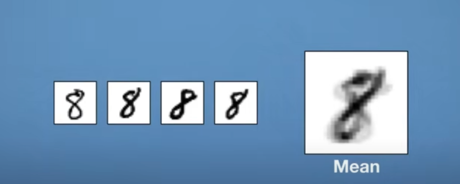
we have different 8 image where we get mean by adding all pixel and divide by no of image we get mean
Variance?
Variance measures spread how far the numbers are from the mean. Formula for population variance: (How far is one variable from its center?)
Example (same data): , mean
- Differences from mean: , , ,
- Squares:
- Average:
Variance here = 5.
CoVariance
Covariance is a statistical measure of how two random variables change together
- If they tend to increase together, the covariance is positive.
- If one increases while the other decreases, the covariance is negative.
- If they are unrelated, the covariance is close to zero.
Covariance tells us the direction of a relationship but not the strength. (That’s what correlation does more on that later.)
Formula of Covariance
For two random variables and , the population covariance is:
- : the ith data points
- : means of X and Y
- : number of data points
For the sample covariance, we divide by instead of :
What Does Covariance Really Mean?
Let’s break down this formula:
-
tells us how far is from the mean of .
-
tells us the same for .
-
Multiply them → if both deviations are positive or both are negative, the result is positive (they move together).
-
If one is positive and the other is negative → result is negative (they move in opposite directions).
Then, take the average of all those products. That’s the covariance.
Example:
Let’s say we have data for two variables:
| Student | Hours Studied (X) | Exam Score (Y) |
|---|---|---|
| A | 2 | 65 |
| B | 4 | 70 |
| C | 6 | 75 |
| D | 8 | 85 |
| E | 10 | 95 |
Step 1: Calculate the Means
Step 2: Use Formula
Now compute each term :
| X | Y | X−XˉX - \bar{X} | Y−YˉY - \bar{Y} | Product |
|---|---|---|---|---|
| 2 | 65 | -4 | -13 | 52 |
| 4 | 70 | -2 | -8 | 16 |
| 6 | 75 | 0 | -3 | 0 |
| 8 | 85 | 2 | 7 | 14 |
| 10 | 95 | 4 | 17 | 68 |
Sum of products =
Sample size = 5 → use sample covariance (divide by 4):
It’s a positive number, so:
- As hours studied increases, exam score tends to increase.
- The number 37.5 itself doesn’t say how strong the relationship is, just that they’re positively related.