Markov Chain

Philioshopy

Plato’s Perfect Forms

Imagine Plato in ancient Greece, 2000 years ago. He asked: Why do we all understand what a “circle” is if we’ve never seen a perfect one?

His answer: Reality has two layers:

• The imperfect world we perceive (wobbly circles, rough shapes)

• The perfect world of abstract ideals (a true circle with infinite precision)

We can reason about perfect circles mathematically even though they don’t physically exist.

Why is this relevant? Fast forward 2000 years: mathematicians realized that randomness also has hidden perfect forms  we call them probability distributions. A coin flip seems random, but underneath, there’s a perfect mathematical structure (50-50 distribution) that emerges when you repeat it enough times.

 Randomness Is Predictable (Bernoulli’s Urn)

Bernoulli’s thought experiment (1700s):

Imagine an urn with 3000 white pebbles and 2000 black pebbles (unknown to you). You reach in blindly and pull one pebble, write down the color, and return it. You repeat this 100 times, then 1000 times, then 10,000 times.

What do you observe?

Number of Draws	White Ratio	Black Ratio	Approaching…
100 draws	58%	42%	❌ Off by 8%
1,000 draws	59.5%	40.5%	✓ Getting closer
10,000 draws	60.1%	39.9%	✓✓ Very close
100,000 draws	60.02%	39.98%	✓✓✓ Nearly exact

The magic: Your observed ratio (from random draws) converges to the true probability (3:2 = 60:40).

The Intuition

Randomness isn’t chaos — it’s just noise that averages out. Think of it like this:

• One coin flip is unpredictable (heads or tails?)
• But 1000 coin flips? You’ll get ~500 heads and ~500 tails (the bell curve smooths out randomness)
• 1 million flips? Even closer to 50-50

This is foundational to all statistics: If you survey 1,000 people randomly, their preferences won’t be perfect, but they’ll be representative enough of the whole population.

The Challenge — What About Dependent Events? (Nekrasov vs. Markov)

Andrey Markov responded with a brilliant insight:

“You’re right that dependent events are different. But they’re not lawless — they follow different predictable patterns.”

He created a mathematical framework to prove that even when events depend on the past, they can still converge to stable, predictable distributions.

This was a paradigm shift: Dependence doesn’t destroy predictability; it just changes the structure.

 From Markov Chains to Language Models (Shannon to GPT)

Claude Shannon’s Breakthrough

Claude Shannon (1916-2001), the father of Information Theory, made a genius observation:

“English text isn’t random. Each letter strongly depends on the previous letter.”

He wasn’t thinking about AI — he was thinking about efficient communication and compression. He realized:

• “Q” is almost always followed by “U” (dependence!)
• “TH” is a common pair, but “XQ” never appears
• Letter frequencies aren’t independent

Shannon’s Solution: Markov Chains for Text

Shannon built a Markov-chain-based language model by analyzing books and learning transition probabilities.

Example probabilities he might have found:

• P(H | T) = very high (T → H is common: “the”)
• P(E | T) = lower (but still common)
• P(Z | T) = near zero (almost never happens)

Then he asked the model to generate text:

Generated text (order 2 — each letter depends on previous letter):

“TOMANREVEDT TORE BRR NIGHTTIN MTRE PTOROORMODS”

Not English, but it starts looking like it! The model learned statistical patterns.

With higher order (more context):

“THE GENERATED RANDOM TEXT FOR THE PROOF SEEMS TO BE…”

Markov chain

A Markov chain is a mathematical system that moves between states, step by step, over time.

Each time it moves:

• It chooses its next state based only on where it is now,
• Not on how it got there.

In other words, the past doesn’t matter only the present determines the future

Markov chains are used when the future only depends on the present:

This property is called the Markov Property.

Example

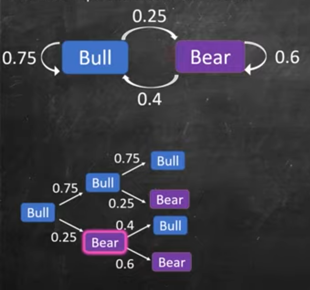
• Bull (B) → Market goes up
• Bear (R) → Market goes down

Transition probabilities:

• If today is Bull, then:
  • 0.75 chance tomorrow is Bull again
  • 0.25 chance tomorrow is Bear
• If today is Bear, then:
  • 0.60 chance tomorrow is Bear again
  • 0.40 chance tomorrow is Bull

That gives us this transition matrix:

$P=\left[\begin{array}{cc}0.75& 0.25\\ 0.40& 0.60\end{array}\right]$

Where:

• Row 1 = “today = Bull”
• Row 2 = “today = Bear”
• Column 1 = “tomorrow = Bull”
• Column 2 = “tomorrow = Bear”

It is nothing but Adjacency Matrix representing the directed graph

Let’s say you know today’s state (a vector):

v_0 = [1, 0]

→ means: 100% chance it’s Bull today, 0% Bear.

Then:

$$\begin{gathered} v_1=v_{0}P=[1,0] \\ \left[\begin{array}{cc}0.75& 0.25\\ 0.40& 0.60\end{array}\right]=[0.75,0.25] \end{gathered}$$

That’s your next-day probabilities:

• 75% chance Bull
• 25% chance Bear

Now apply the matrix again:

$$v_2=v_{1}P=[0.75,0.25]P=[0.65,0.35]$$

So after two weeks, 65% chance of being Bull.

Tree Diagram

The tree diagram in the video is just a visual version of multiplying probabilities manually.

It did:

Bull → Bull → Bull: 0.75 × 0.75 = 0.5625 Bull → Bear → Bull: 0.25 × 0.40 = 0.10

Add both → 0.6625 (≈ 66%) Bull after 2 weeks

The matrix version automates this:

• Instead of expanding trees,
• You multiply matrices repeatedly.

Stationary Distribution

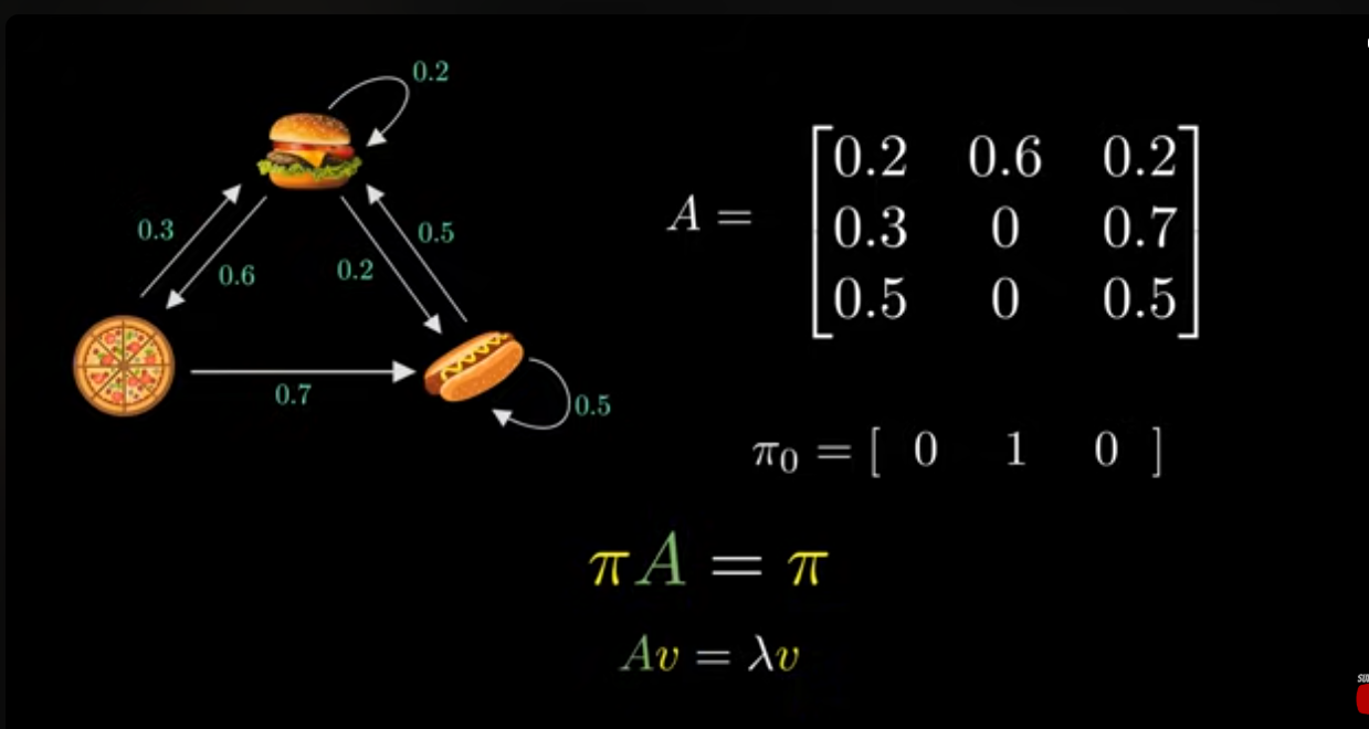
first - burger second piza thrid hot dog

Where PIE is the probablity of putting piza on next day if we keep calculating on until infinity we get same probablity of we give that what Stationary Distribution

Now imagine doing this forever:

$$v_n=v_0{P}^n$$

As to infinity, often the probabilities settle into a fixed pattern they stop changing.

That stable vector is called the stationary distribution, denoted by pie

It satisfies: $\pi P=\pi$

and the probabilities sum to 1. For our example, solving it gives:

$$\pi =[0.615,0.385]$$

Meaning:

• Long-term, 61.5% of weeks are Bull
• 38.5% are Bear

So even though it bounces randomly, it stabilizes statistically.

• The stationary vector $\mathbf{\pi }$ is the left eigenvector for eigenvalue 1.

• All other eigenvalues (in magnitude) govern how fast the chain “forgets” its start smaller second eigenvalue magnitude → faster mixing.

• The memoryless property is what makes Markov chains tractable: the entire future depends only on the current row of P.

Concept	Meaning
State	Current situation (city, weather, stock type)
Transition probability	Chance of moving from one state to another
Transition matrix (P)	Mathematical table encoding all probabilities
Markov Property	Future depends only on present, not past
vₙ = v₀ Pⁿ	Predicts the distribution after n steps
Stationary distribution	Long-run stable probabilities that no longer change

Other models

Model	Key Idea
Higher-order Markov Chain	Depend on last k steps, not just 1.
Hidden Markov Model (HMM)	Introduce hidden “true” states and noisy observations.
Markov Decision Process (MDP)	Add actions and rewards to model decision-making.
Recurrent Neural Networks (RNNs)	Learn to compress long-term context into a hidden state (still a Markov process in latent space).
Transformers (like GPT)	Drop the Markov assumption; look at all past tokens directly.

Code example

# State: 0=Sunny, 1=Rainy
transitions = {
    0: {0: 0.8, 1: 0.2},  # From sunny: 80% stay sunny, 20% rain
    1: {1: 0.6, 0: 0.4}   # From rainy: 60% stay rainy, 40% sunny
}
 
current_state = 0  # Start sunny
history = [current_state]
 
for day in range(1000):
    # The Markov property: only current_state matters
    probabilities = transitions[current_state]
    next_state = random.choice(state, p=[probabilities[0], probabilities[1]])
    current_state = next_state
    history.append(current_state)
 
# Check stationary distribution
sunny_days = sum(1 for s in history if s == 0)
print(f"Sunny: {sunny_days/1000:.1%}")  # Will be ~67%
 

NLP example

We’ll treat text as a sequence of tokens (words or characters).

The Markov assumption says:

“The next token depends only on the current one (not the whole history).”

So we’ll:

1. Count how often each word is followed by each other word.
2. Convert those counts into probabilities.
3. Use those probabilities to randomly generate new text.

That’s the simplest possible “language model.”

Let’s start with a tiny dataset so we can see everything by hand:

text = "the cat sat on the mat the cat ate the rat"

Tokens =["the", "cat", "sat", "on", "the", "mat", "the", "cat", "ate", "the", "rat"]

Build transition counts

We go word by word and record what follows what.

Current	Next	Count
the	cat	2
the	mat	1
the	rat	1
cat	sat	1
cat	ate	1
sat	on	1
on	the	1
mat	the	1
ate	the	1
rat	—	0

So we can represent this as a dictionary of lists:

{
  "the": ["cat", "mat", "rat"],
  "cat": ["sat", "ate"],
  "sat": ["on"],
  "on": ["the"],
  "mat": ["the"],
  "ate": ["the"],
  "rat": []
}

Convert counts to probabilities Now we can calculate the probability of each possible next word. Example:

• After “the”: 4 total transitions (2+1+1)
  • P(cat|the) = 2/4 = 0.5
  • P(mat|the) = 1/4 = 0.25
  • P(rat|the) = 1/4 = 0.25 We can store it like:

{
  "the": {"cat": 0.5, "mat": 0.25, "rat": 0.25},
  "cat": {"sat": 0.5, "ate": 0.5},
  "sat": {"on": 1.0},
  "on": {"the": 1.0},
  "mat": {"the": 1.0},
  "ate": {"the": 1.0},
  "rat": {}
}

This is your transition probability table.

Generate new text Algorithm:

1. Pick a random starting word (say “the”).
2. Sample the next word based on probabilities.
3. Repeat until no next word or we reach desired length.

import random
from collections import defaultdict
 
# Sample training text
text = """
the cat sat on the mat and the cat ate a rat the rat ran away from the cat
"""
 
# STEP 1: Tokenize (split into words)
words = text.strip().split()
 
# STEP 2: Build transition probabilities
transitions = defaultdict(list)
for i in range(len(words) - 1):
    curr_word = words[i]
    next_word = words[i + 1]
    transitions[curr_word].append(next_word)
 
# STEP 3: Generate new text
def generate_text(start_word, length=15):
    word = start_word
    output = [word]
    for _ in range(length - 1):
        if word not in transitions:
            break
        word = random.choice(transitions[word])
        output.append(word)
    return " ".join(output)
 
# Example usage
print(generate_text("the", 20))
 
 

Hidden Markov Model