Probability

├── Probability
│   ├── Random Variables
│   │   ├── Discrete Random Variables               
│   │   └── Continuous Random Variables             
│   ├── Probability Distributions
│   │   ├── Bernoulli
│   │   ├── Binomial
│   │   ├── Gaussian (Normal)
│   │   ├── Poisson
│   │   ├── Uniform
│   │   ├── Exponential  
│   │   ├── Multinomial  
│   │   ├── Beta         
│   │   ├── Dirichlet    
│   │   └── Categorical  
│   ├── Expectation
│   ├── Variance
│   ├── Covariance
│   ├── Correlation      
│   ├── Joint Probability
│   ├── Marginal Probability                        
│   ├── Conditional Probability
│   ├── Bayes Theorem
│   ├── Independence     
│   ├── Law of Large Numbers                        
│   ├── Central Limit Theorem                       
│   ├── Maximum Likelihood Estimation (MLE)         
│   ├── Maximum A Posteriori (MAP)                  
│   └── Probability Density / Mass Functions        

probability

Intuition: A probability problem is about events (sets of outcomes), not a single “mystical” outcome. The sample space S is “everything that could possibly happen.” An event E is a subset of S

If every outcome in a finite sample space S is equally likely, the probability of event E is

$$\boxed{P(E)=\frac{|E|}{|S|}}$$

where $|\cdot |$ counts outcomes.

Examples

• Two fair coin flips: $S=\{HH,HT,TH,TT\}$. Event $A$ = “at least one head” = $\{HH,HT,TH\}$. So $P(A)=3/4$.

• Draw one card from standard 52-card deck: Event “king” has 4 outcomes, so $P(\text{king})=4/52=1/13$.

Why is counting outcomes enough only when outcomes are equally likely? Because probability is a weighting if outcomes differ in likelihood you must weight them differently (that’s when PMFs/PDFs come in).

let say we have coin where there is high probablity of getting head because the coin has over weight on head side which need to consider on calculating the probabliity which is PMF,PDF

Axioms of probability (Kolmogorov)

Kolmogorov’s three axioms for a probability measure $P$ on a sample space $S$:

1. Non-negativity: $P(A)\ge 0$ for every event $A$.

2. Normalization: $P(S)=1$.

3. Countable additivity: For disjoint events $A_1,A_2,\dots$ (pairwise disjoint),

$$P\left(\bigcup _{i=1}^{\infty }{A}_i\right)=\sum _{i=1}^{\infty }P(A_i).$$

Immediate consequences (proof sketches)

• $P(\varnothing )=0$: because $S$ and $\varnothing$ are disjoint and $P(S)=1$.

• Monotonicity: If $A\subseteq B$ then $P(A)\le P(B)$. (Because $B$ is union of $A$ and $B\setminus A$, both nonnegative.)

• For two events $A,B$:

$$\boxed{P(A\cup B)=P(A)+P(B)-P(A\cap B)}$$

(derived by splitting overlapping part once).

Axioms are simple but powerful many neat identities are immediate once you know how to partition sets.

Notation

• Complement: $A^c=\Omega \setminus A$
• Union: $A\cup B$
• Intersection: $A\cap B$
• Empty set: $\varnothing$

Set Theory Operations

Union $A\cup B$

• Collects outcomes from either A or B (or both).
• Analogy: two groups of friends → union = everyone who is in at least one of the groups.
• Probability: $P(A\cup B)$ = “chance that A happens, or B happens, or both.”

Intersection $A\cap B$

• Outcomes common to both sets.
• Analogy: friends in both your school and football team.
• Probability: $P(A\cap B)$ = “chance that A and B happen simultaneously.”

Complement $A^c$

• Everything in the sample space not in $A$.
• Analogy: if A = “it rains today,” then $A^c$ = “it does not rain today.”
• Probability: $P(A^c)=1-P(A)$.

Collections of Sets

• Mutually exclusive (disjoint): cannot overlap → $A_i\cap A_j=\varnothing$.

Example: rolling a die → “even” and “odd” outcomes.

• Collectively exhaustive: together they cover everything → ${\bigcup }_i{A}_i=S$.

Example: “even” or “odd” outcomes cover all die rolls.

• Partition: both mutually exclusive and collectively exhaustive.

Example: die → $\{1\},\{2\},\{3\},\{4\},\{5\},\{6\}$.

→ partitions are very powerful because they let us break probability into disjoint chunks → critical for Bayes’ theorem later.

The Notion of Probability

Relative Frequency (intuitive definition)

$$P(A)=\underset{n\to \infty }{\lim }\frac{\text{Number of times A occurs}}{n}.$$

• Works nicely for finite sample spaces (coins, dice).

• Intuition: repeat an experiment many times → fraction of times A occurs “settles down.” Limitation: doesn’t extend cleanly to infinite/continuous cases.

• Example: choosing a random number between 0 and 1.

• What’s the probability of picking exactly 0.5? Relative frequency says “0” (because infinite possibilities).

• But the formal measure-theoretic definition handles this: single points in continuous distributions indeed have probability 0.

Probability Measure

A probability measure is a function:

$$P:\mathcal{F}\to [0,1]$$

where $\mathcal{F}$ is a collection of events (subsets of sample space).

Properties:

• Assigns 0 to impossible event, 1 to certainty.
• Behaves additively over disjoint events.
• General enough to handle both finite and infinite spaces.

Types

1. Marginal Probability

The probability of a single event happening, without considering any other events.

Formula:

$$P(A)=\frac{\text{Number of outcomes favorable to A}}{\text{Total outcomes}}$$

Example:* If 60 out of 100 students like ice cream, then:

$P(\text{Ice Cream})=\frac{60}{100}=0.6$

2. Union Probability (OR)

Probability that at least one of two (or more) events happens.

$P(A\cup B)=P(A)+P(B)-P(A\cap B)$

• 60 students like ice cream.
• 40 students like cake.
• 20 like both.

Then:

$$P(\text{Ice Cream or Cake})=\frac{60}{100}+\frac{40}{100}-\frac{20}{100}=0.8$$

So, 80% like at least one.

3. Intersection Probability (AND)

Probability that both events happen at the same time.

$P(A\cap B)=\frac{\text{Number of outcomes where A and B occur}}{\text{Total outcomes}}$

• Example: If 20 students out of 100 like both ice cream and cake:

$$P(\text{Ice Cream AND Cake})=\frac{20}{100}=0.2$$

4. Conditional Probability

Probability of one event given that another event has already happened.

$P(A|B)=\frac{P(A\cap B)}{P(B)}$

Example: If I tell you a student likes ice cream (60 students), what is the probability they also like cake (20 students like both)?

$$P(\text{Cake | Ice Cream})=\frac{20/100}{60/100}=\frac{20}{60}=0.33$$

5. Complement Probability

Probability that an event does NOT happen.

$P(A^c)=1-P(A)$

Example: If 60% like ice cream, then the probability a student does not like ice cream is:

$$P(\text{Not Ice Cream})=1-0.6=0.4$$

Sum rule

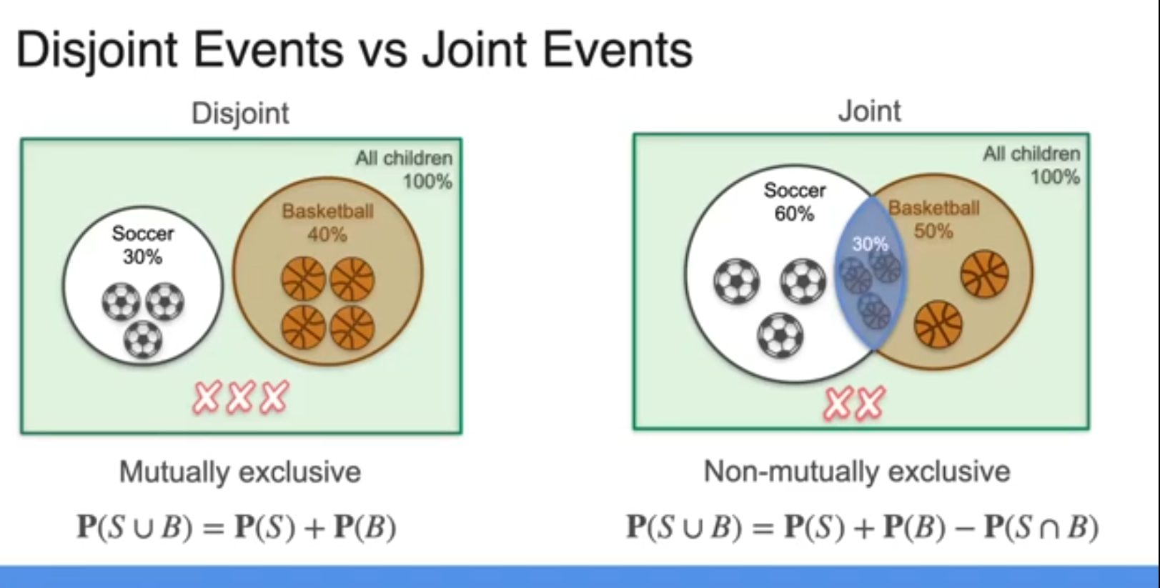
Disjoint Events (Mutually Exclusive)

Two events are disjoint if they cannot happen at the same time.

Example: In a coin toss, the event Heads and the event Tails are disjoint you can’t get both on a single toss.

• Rule: $P(A\cup B)=P(A)+P(B)$

Because there is no overlap, we just add the probabilities.

Joint Events (Overlapping)

Two events are joint if they can occur together. Example: A student can play both football and basketball.

• Rule: $P(A\cup B)=P(A)+P(B)-P(A\cap B)$

We subtract $P(A\cap B)$ (the intersection) to avoid double counting the students who do both.

Dependent and Independent Events

Two events are independent if the outcome of one does not affect the outcome of the other.

• Rule: $P(A\cap B)=P(A)\cdot P(B)$

This means the probability of both happening is just the product of their individual probabilities.

• Tossing a coin and rolling a die.
• Whether the coin lands heads has nothing to do with what number shows up on the die.
• So, $P(\text{Heads and 4})=P(\text{Heads})\times P(\text{4})=\frac{1}{2}\times \frac{1}{6}=\frac{1}{12}$.

Dependent Events Two events are dependent if the outcome of one affects the outcome of the other.

• Rule: $P(A\cap B)=P(A)\cdot P(B|A)$

Here, $P(B|A)$ means the probability of $B$ happening given that $A$ has already happened.

• Drawing cards from a deck without replacement.
• Suppose you draw one card and it’s an Ace. Now the probability of drawing another Ace changes, because only 3 Aces are left out of 51 cards.
• That’s a dependent situation.

Conditional probablity

It’s the probability of an event given that another event has already happened.

Notation: $P(A|B)$

This means “the probability of event $A$ occurring, given that event $B$ has occurred.”

$$P(A|B)=\frac{P(A\cap B)}{P(B)}\text{(as long as P(B)>0)}$$

• Idea: We restrict our universe to only cases where $B$ happens, and then ask: within that restricted world, how often does $A$ also happen?

Total deck = 52 cards. Event $A$: Draw a King. Event $B$: Draw a Spade.

We want $P(A|B)$: probability of drawing a King given the card is a Spade.

• How many Spades? 13.
• How many of those are Kings? Just 1 (King of Spades). $P(A|B)=\frac{1}{13}$

If $A$ and $B$ are independent, then: $P(A|B)=P(A)$ also

$P(A\cap B)=P(A)\cdot P(B)$

If they are independent

Because knowing $B$ happened doesn’t change the probability of $A$.

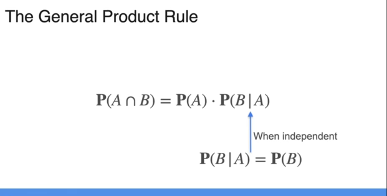
Example

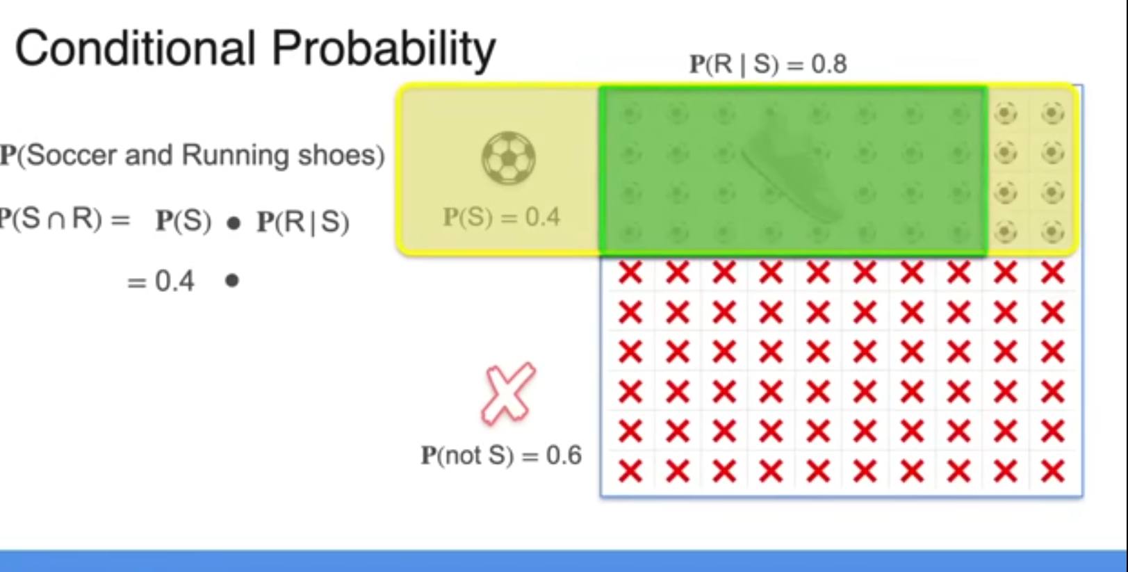Joint probability = “both happen” $P(S\cap R)$

Conditional probability = “one happens, given the other already happened”

$$P(R\mid S)=\frac{P(S\cap R)}{P(S)}(P(S)>0)$$

Link between them (always true):

$$P(S\cap R)=P(S)P(R\mid S)$$

Given:

$P(S)=0.4$ (40% play soccer), $P(R\mid S)=0.8$ (among soccer players, 80% wear running shoes).

Find: $P(S\cap R)$ (play soccer and wear running shoes).

Method 1 — Formula

$$P(S\cap R)=P(S).P(R\mid S)=0.4\times 0.8=0.32$$

Answer: $P(S\cap R)=0.32$ (32% of all students do both).

• $P(S\cap R)$ is about the whole population (what percent of everyone has both).

• $P(R|S)$ is about the restricted group (among soccer players only, how many have running shoes).

Bayes’ Theorem

Random varaiable

A random variable (RV) is simply a function that assigns a number to each outcome of a random experiment.

A random variable is just a way to assign a number to something uncertain in real life → so we can measure, analyze, and make decisions.

Example

Daily Rainfall

• Every day, there’s some rainfall in your city.
• Some days: 0 mm (no rain).
• Some days: 5 mm, 10 mm, maybe 100 mm during storms.
• The exact rainfall tomorrow is uncertain → that’s the randomness.

We define a random variable $R$: $R=\text{“rainfall amount tomorrow (in mm)”}$

• If tomorrow rains 20 mm → $R=20$.
• If no rain → $R=0$.

Now we can ask useful questions:

• What’s the average rainfall in August? ($E[R]$)
• What’s the probability rainfall exceeds 50 mm tomorrow? ($P(R>50)$)

This is how meteorologists make forecasts.

Probability Distribution

A probability distribution tells us how the probabilities are spread across the values of a random variable.

In other words:

• A random variable says “What numbers are possible?”
• A probability distribution says “How likely is each number?”

A fair coin toss

Outcomes: {Head, Tail} Probabilities: {0.5, 0.5} This is a probability distribution because:

• All probabilities are between 0 and 1.
• They add up to 1.

Rolling a fair die

Outcomes: {1,2,3,4,5,6} Probabilities: {1/6 each} Distribution: $P(X=1)=\frac{1}{6},P(X=2)=\frac{1}{6},\dots ,P(X=6)=\frac{1}{6}$

Two Main Types of Probability Distributions

Discrete Distribution

• Outcomes are countable (like coin toss, dice, number of students).
• Probabilities are assigned to each outcome separately.

Types

1. Bernoulli Distribution
   • One trial, success/failure.
   • Building block.
2. Binomial Distribution
   • Repeated Bernoulli trials.
   • Example: number of heads in 10 tosses.
3. Geometric Distribution
   • Number of trials until first success.
   • Example: “How many times do I toss until I see heads?”
4. Negative Binomial Distribution
   • Number of trials until k-th success.
   • Example: “How many shots until I hit 3 goals?”
5. Poisson Distribution
   • Models rare events in a fixed time/space.
   • Example: earthquakes per year, calls per hour at a call center.

Continuous Distribution

• Outcomes come from a range of numbers (like height, weight, time).
• We don’t assign probability to a single point, but to intervals.
• Use curves instead of bars.

Types

1. Uniform Distribution
   • All values equally likely in an interval.
   • Example: picking a random number between 0 and 1.
2. Normal (Gaussian) Distribution
   • Bell curve, most famous.
   • Example: heights, exam scores.
3. Exponential Distribution
   • Time until an event happens (like waiting time).
   • Example: time between bus arrivals.
4. Gamma Distribution
   • Generalization of exponential.
   • Example: total waiting time for multiple events.
5. Chi-Square Distribution
   • Special case of Gamma.
   • Common in hypothesis testing.
6. t-Distribution
   • Similar to normal but heavier tails.
   • Example: used in small-sample statistics.
7. F-Distribution
   • Ratio of variances.
   • Example: ANOVA tests.

Rules of a Probability Distribution

For a random variable $X$:

1. $P(X=x)\ge 0$ (no negative probabilities).

2. Sum of all probabilities = 1 (for discrete). $\sum P(X=x)=1$ Or, for continuous: $\int f(x)dx=1$

Probability Mass Function

• Used when outcomes are discrete (countable).
• It tells the probability of each exact outcome.

Example: Roll a die 🎲 $P(X=k)=\frac{1}{6},k=1,2,3,4,5,6$

This is the PMF. It satisfies: ${\sum }_{k=1}^{6}P(X=k)=1$

Think of PMF as: “What’s the chance of getting exactly this outcome?”

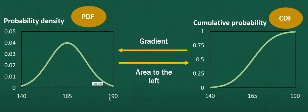
PDF – Probability Density Function (Continuous case only)

• Used when outcomes are continuous (uncountable).
• Probability at one exact point = 0 (e.g., chance of being exactly 160.00000 cm tall is 0).
• Instead, PDF gives us a curve.
• Probability is found by the area under the curve between two points.

Example: Heights of students follow a normal curve.

$$P(160\le X\le 170)={\int }_{160}^{170}f(x)dx$$

Think of PDF as: “The height of the curve that shapes probabilities.”

CDF – Cumulative Distribution Function (Both discrete & continuous)

cumulative distribution function of X, which is a function that represents the probability that X is less than or equal to any value a and is equal to the sum of all the probabilities for X that are less than or equal to a. In probability notation, the cumulative distribution function (cdf) of X, is written as F(a) = !P (X = x).

• CDF = Probability that the variable is less than or equal to some value. $F(x)=P(X\le x)$

• We add the probablity of 1.. to n if you see the below image where we have first have probablity of getting 0 then p(x>1) then p(x>2) which is p(0) + p(1) + p(2)

• PMF → Discrete → Probability of exact value.

• PDF → Continuous → Density curve, probability via area.

• CDF → Both → Probability up to a value.

The CDF show how much probablity the variables has accumulated untill a certaiin value

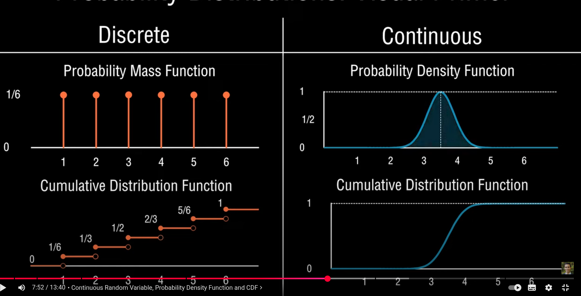Discrete CDF (bottom left): “As I move right, I’m accumulating all the probability I’ve passed”

Continuous PDF (top right): “Here’s the ‘shape’ of where values cluster - calculate areas for probabilities”

• The curve shows where values are more or less likely
• Peak around 3 = values near 3 are most common
• Tails near 1 and 6 = extreme values are rare
• CRITICAL: The HEIGHT is NOT probability!
• We CANNOT say “probability at exactly 3.0000… is X”
• Instead: AREA under the curve = probability
• The shaded blue area = probability that X falls in that range

Continuous CDF (bottom right): “As I move right, I’m smoothly accumulating all the probability in a continuous way”

• Same concept as discrete CDF - “What’s P(X ≤ x)?”
• At x=1: CDF ≈ 0 (almost nothing below 1)
• At x=3: CDF ≈ 0.5 (50% of values are below 3) — see the dotted line!
• At x=6: CDF ≈ 1 (almost everything below 6)
• Why smooth? Because the variable is continuous. As x increases even slightly, the cumulative probability increases smoothly (no sudden jumps).

Expected Value (Mean)

• What it is: The expected value is the long-term average or “center” of the distribution of a random variable. It’s the value you’d expect to get if you repeated an experiment a large number of times.

• Formula: For a discrete random variable ( X ), if ( x_1, x_2, …, x_n ) are the possible values of ( X ), and ( p_1, p_2, …, p_n ) are the probabilities of those values, the expected value is: $E(X)={\sum }_{i=1}^n{x}_i\cdot p_i$

• Example: If you roll a fair six-sided die, the expected value would be: $E(X)=\frac{1}{6}(1)+\frac{1}{6}(2)+\frac{1}{6}(3)+\frac{1}{6}(4)+\frac{1}{6}(5)+\frac{1}{6}(6)=3.5$ This means that, on average, if you roll the die many times, the expected value of the rolls will be around 3.5.

Mean and variance

A probability distribution tells us:

• all the possible values a random variable can take,
• and how likely each value is.

But a whole distribution is a lot of information.

So we use summary statistics to capture the “essence” in just a couple of numbers.

That’s where mean and variance come in.

Mean

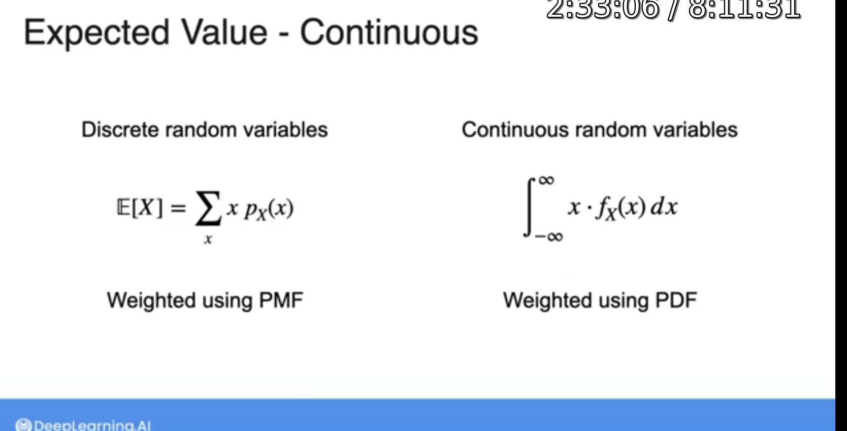
The mean of a distribution is the center where outcomes “average out” if you repeat the experiment many times.

• It’s called expected value because it’s the long-term average.

For discrete random variable $X$: $\mu =E[X]={\sum }_{x}x\cdot P(X=x)$

For continuous random variable $X$: $\mu =E[X]={\int }_{-\infty }^{\infty }x\cdot f(x)dx$

(where $f(x)$ is the PDF).

Example: Toss a fair coin, let $X=1$ if heads, $0$ if tails. $E[X]=0\cdot 0.5+1\cdot 0.5=0.5$

So on average, you expect “half heads”.

Variance (Spread)

• The variance measures how spread out the values are from the mean.
• If all outcomes are very close to the mean, variance is small.
• If outcomes are scattered far away, variance is large.

For discrete: $Var(X)=E[(X-\mu {)}^2]={\sum }_x(x-\mu {)}^2\cdot P(X=x)$

For continuous: $Var(X)={\int }_{-\infty }^{\infty }(x-\mu {)}^{2}f(x)dx$

Example: Coin toss $X$ (same as before).

Mean $E[X]=0.5$.

Variance:$Var(X)=(0-0.5{)}^2\cdot 0.5+(1-0.5{)}^2\cdot 0.5=0.25$

So the coin toss outcomes vary around 0.5 with variance 0.25.

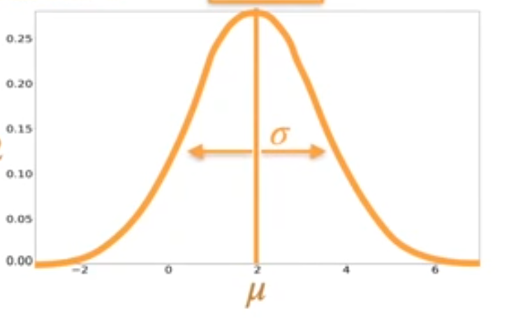
NOTE: So we can control the curve using mean and variance

Standard Deviation (SD)

The standard deviation (σ) is just the square root of variance. $\sigma =\sqrt{Var(X)}$

Why take the square root?

Because variance is in “squared units” (e.g., cm² if measuring height), while SD brings it back to the same unit as the data (cm).

The spread of values around the expected value, in the same units as the original variable.

Permutation and combination

Permutation (order matters)

Number of ways to arrange $r$ objects out of $n$:

$$P(n,r)=\frac{n!}{(n-r)!}$$

Use this when the sequence or arrangement matters. Example: Arranging 3 students out of 10 in a line.

Combination (order doesn’t matter)

Number of ways to choose $r$ objects out of $n$:

$$C(n,r)=\left(\genfrac{}{}{0ex}{}{n}{r}\right)=\frac{n!}{r!(n-r)!}$$

Use this when only the group matters, not the order.

Example: Selecting 3 students out of 10 to form a committee.

Probability formula

$$P(\text{Event})=\frac{\text{Number of favorable outcomes}}{\text{Total outcomes}}$$

• Use permutation if both numerator & denominator involve ordered outcomes.
• Use combination if both are unordered.

Example 1: Combination probability

From a 52-card deck, what’s the probability of drawing 2 aces in a 5-card hand?

• Total 5-card hands: $\left(\genfrac{}{}{0ex}{}{52}{5}\right)$
• Favorable: choose 2 aces from 4 and 3 other cards from 48: $\left(\genfrac{}{}{0ex}{}{4}{2}\right)\left(\genfrac{}{}{0ex}{}{48}{3}\right)$

$P=\frac{\left(\genfrac{}{}{0ex}{}{4}{2}\right)\left(\genfrac{}{}{0ex}{}{48}{3}\right)}{\left(\genfrac{}{}{0ex}{}{52}{5}\right)}$

Permutation probability

A locker has a 3-digit code using digits 0–9 (repetition not allowed). What’s the probability of guessing it right on the first try?

• Total possible codes: $P(10,3)=10\cdot 9\cdot 8$
• Favorable: only 1 correct code $P=\frac{1}{10\cdot 9\cdot 8}=\frac{1}{720}$

Situation	Example	Formula
Permutation (order matters)	First, second, third prize winners in a race	${}^n{P}_r=\frac{n!}{(n-r)!}$
Combination (order doesn’t matter)	Choosing 3 students for a team	${}^n{C}_r=\frac{n!}{r!(n-r)!}$

Binomial Distribution

For a situation to qualify for a binomial distribution, it needs to meet these conditions:

1. Fixed Number of Trials: The number of trials must be set ahead of time and known (e.g., flipping a coin 10 times).

2. Two Possible Outcomes: Each trial must result in either a success or a failure (e.g., heads or tails, yes or no).

3. Constant Probability of Success: The probability of success ( p ) must be the same for each trial (e.g., if flipping a fair coin, the probability of heads is always 0.5).

4. Independent Trials: The outcome of one trial should not affect the outcome of any other trial.

The Probability Mass Function (pmf) for Binomial Distribution

• The pmf for a binomial random variable ( X ) is used to calculate the probability that ( X ) takes on a specific value (i.e., the probability of getting exactly ( x ) successes in ( n ) trials). The formula is:

$$P(X=x)=\left(\genfrac{}{}{0ex}{}{n}{x}\right)p^x(1-p{)}^{n-x}$$

Where:

• ( \binom{n}{x} ) (read “n choose x”) is the number of ways to choose ( x ) successes out of ( n ) trials.
• ( p ) is the probability of success on a single trial.
• ( 1 - p ) is the probability of failure on a single trial.
• ( x ) is the number of successes you are interested in, and ( n ) is the total number of trials.

binomial probability formula is a powerful tool for modeling scenarios where you’re counting the number of successes in a fixed number of independent trials. The formula is built from a few foundational concepts: combinatorics, probability, and the multiplication rule of independent events.

Normal Distribution

The normal distribution is a bell-shaped, symmetric curve that shows how data is spread out. It’s used to model many real-life things like test scores, heights, weights, etc.

• Shape: Bell-shaped and symmetric around the center.
• Center: The mean (µ) is the middle point where the peak of the curve is.
• Spread: The standard deviation (σ) measures how spread out the values are.
  • Smaller σ → thinner, taller curve.
  • Larger σ → wider, flatter curve.

Example Think about something like human height. If we measured 1000 people, you’d see this:

• Most people are somewhere around the average (say 170 cm).
• A few are shorter.
• A few are taller.
• Very few are much shorter or much taller.

If we graphed that, it makes a hill shape a bell curve.

Intuition: The normal distribution is nature’s way of saying: “Most things are average. Extreme things are rare.”

Axis

• X-axis (horizontal) = the values of the variable you’re measuring
  → e.g. height, test score, weight, etc.
  This is what you’re interested in.
• Y-axis (vertical) = the probability density
  → tells you how likely each value on the X-axis is.
  It shows how “dense” the data is at each point — NOT the actual probability.

The Z-score answers this:

“How far away am I from average”

So…

• Z = 0 → You’re exactly average.
• Z = +1 → You’re one step (SD) above average.
• Z = –1 → You’re one step (SD) below average.
• Z = +3 → You’re very rare and high (only 0.1% of people are here).
• Z = –2 → You’re rare and low.

Resources

• Probability Distribution Functions (PMF, PDF, CDF)
• https://seeing-theory.brown.edu/#4thPage