Text classifcation NLP

Naive Bayes

To classify a piece of text as being either positive or negative sentiment. If the word “amazing” appears, what is the probability that that document is positive? Let’s use Bayes’ theorem.

$P (p os i t i v e ∣" ama z in g ") = P (" ama z in g "∣ p os i t i v e) P (p os i t i v e) P (" ama z in g ")$

We can work out the 3 terms on right side of the equation as follows:

P(positive) - count how many documents are positive and divide by the total number of documents,
P(“amazing”) - count how many times the word “amazing” appears in the corpus and divide by the total number of words,
P(“amazing”|positive) - out of all the positive documents, count how many times the word “amazing” appears and divide by the number of words in the positive documents.

So we converted the question from inferring the sentiment into a matter of working out the proportions a word appears in different documents. And this is something computers can do very quickly. But what do we do if we want to condition on a whole document and not just a single word? Let’s see below.

Multinomial NB: models word counts (good for typical bag-of-words).
Bernoulli NB: models word presence/absence (binary features).

How it works

We want to compute:

P (Class ∣ Words) = \frac{P ( Words ∣ Class ) , P ( Class )}{P ( Words )}

Since (P(\text{Words})) is the same for all classes, we only need:

P (Words ∣ Class), P (Class)

The “Naïve” assumption: Words are conditionally independent given the class. So:

P (w_{1}, w_{2}, \dots, w_{n} ∣ Class) = i \prod P (w_{i} ∣ Class)

How text features fit in

Step 1: Turn text into numbers

You can use:

CountVectorizer: number of times each word appears.
TfidfVectorizer: same, but scaled by rarity (IDF).

Each document becomes a vector of word strengths.

Step 2: Compute probabilities

For each class (e.g., spam or ham):

Estimate how frequently each word appears in that class.
The classifier learns (P(w_i \mid \text{Class})) from the training data.

Then for a new document:

Look up each word’s probability under each class.
Multiply (or sum logs) to find which class is more probable.

Why IDF helps (intuition)

Let’s use a tiny example.

Document	Text	Label
D₁	“buy cheap pills now”	spam
D₂	“buy cheap watches”	spam
D₃	“meeting schedule update”	ham

Vocabulary

$$buy, cheap, pills, now, watches, meeting, schedule, update$$

Case 1: Without IDF (plain counts)

Common word like “buy” appears in both spam and ham → its count will influence both equally.

But “pills” appears only in spam → it should have much higher importance.

Naïve Bayes with raw counts might under-emphasize that difference, because every word is treated equally frequent.

Case 2: With TF-IDF

IDF down-weights words that appear in many documents, and up-weights words that appear in few documents.

“buy” → appears in 3 docs → low IDF (common, less useful)
“pills” → appears in 1 doc → high IDF (rare, more discriminative)
“meeting” → appears in 1 doc (ham) → high IDF but used by other class

So in TF-IDF space:

buy    → small weight (common)
pills  → large weight in spam
meeting → large weight in ham

That means:

Spam docs will have high TF-IDF for “pills”, “cheap”, etc.
Ham docs will have high TF-IDF for “meeting”, “schedule”.

Now Naïve Bayes sees more distinctive numerical patterns per class, so classification becomes cleaner.

Mechanistic view

Input: matrix X from TfidfVectorizer
- Each row = document
- Each column = word’s TF-IDF
Model: MultinomialNB (or BernoulliNB)
- Learns (P(w_i \mid \text{Class})) using these weighted values
Prediction: For new doc → compute
$score(Class) = i \sum TFIDF (w_{i}) \times lo g P (w_{i} ∣ Class) + lo g P (Class)$
→ choose class with highest score.

Example

The model uses the TF-IDF matrix X (numbers) and learns how strongly each word (feature) is associated with each class.

Then, for a new document, it computes a score per class using:

score(Class) = i \sum TFIDF (w_{i}) \times lo g P (w_{i} ∣ Class) + lo g P (Class)

Whichever class has the higher score → that’s the predicted class.

Mini example

Let’s pretend we’re classifying two types of messages:

Message	Text	Class
D₁	”buy pills”	spam
D₂	”cheap pills”	spam
D₃	”project meeting”	ham
D₄	”meeting schedule”	ham

Vocabulary (from all docs)

[buy, cheap, pills, project, meeting, schedule]

So there are 6 words → 6 columns.

Step 1: TF-IDF matrix (simplified numbers)

To keep it readable, let’s assign rough TF-IDF values:

Doc	buy	cheap	pills	project	meeting	schedule
D₁ (spam)	0.7	0	0.9	0	0	0
D₂ (spam)	0	0.7	0.9	0	0	0
D₃ (ham)	0	0	0	0.7	0.9	0
D₄ (ham)	0	0	0	0	0.7	0.9

Step 2: Naïve Bayes learns ( P(w_i \mid \text{Class}) )

The model sums TF-IDF weights within each class and normalizes.

| Word | Sum in Spam | Sum in Ham | (P(w|Spam)) | (P(w|Ham)) | |------|--------------|-------------|----------------|---------------| | buy | 0.7 | 0 | 0.7 / (0.7+0.7+0.9+0.9) ≈ 0.19 | 0 | | cheap | 0.7 | 0 | 0.19 | 0 | | pills | 1.8 | 0 | 0.49 | 0 | | project | 0 | 0.7 | 0 | 0.27 | | meeting | 0 | 1.6 | 0 | 0.62 | | schedule | 0 | 0.9 | 0 | 0.35 |

(These are simplified normalized values — just to illustrate that spam words get probability mass in spam, ham words in ham.)

Step 3: Predict a new message

"cheap pills meeting"

TF-IDF (simplified) for this new doc:

Word	TF-IDF
cheap	0.6
pills	0.8
meeting	0.7

Now compute class scores.

Spam score

score(Spam) = 0.6 lo g P (c h e a p ∣ Sp am) + 0.8 lo g P (p i ll s ∣ Sp am) + 0.7 lo g P (m ee t in g ∣ Sp am) + lo g P (Sp am)

Since (P(meeting|Spam)) ≈ 0 (word unseen in spam), this term heavily reduces the score — but smoothing keeps it small, not infinite.

Ham score

score(Ham) = 0.6 lo g P (c h e a p ∣ H am) + 0.8 lo g P (p i ll s ∣ H am) + 0.7 lo g P (m ee t in g ∣ H am) + lo g P (H am)

Here, (P(cheap|Ham)) and (P(pills|Ham)) are near 0 (never seen in ham), but (P(meeting|Ham)) is large.

Step 4: Compare

Spam: big positive contributions from “cheap”, “pills”
Ham: big positive contribution from “meeting”, but zero for others

If the total spam score is higher → classified as spam.

Confusion Matrix

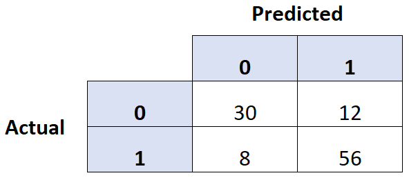
we used to evaluate the classifcation problem where row we have what we excepting and column is what machine predicted

Let say we have class 0 And 1

where below we have how many of 0 class are actullay predicted as 0 is 30 and how many 0 predicted as 1 was 12