DDL Data Definition Language

Command	Purpose	Example
`CREATE DATABASE`	Create database	`CREATE DATABASE shop;`
`DROP DATABASE`	Delete database	`DROP DATABASE shop;`
`CREATE TABLE`	Create table	`CREATE TABLE users (id INT, name VARCHAR(50));`
`DROP TABLE`	Delete table	`DROP TABLE users;`
`TRUNCATE TABLE`	Delete all rows (fast)	`TRUNCATE TABLE users;`
`ALTER TABLE ADD`	Add column	`ALTER TABLE users ADD age INT;`
`ALTER TABLE DROP`	Remove column	`ALTER TABLE users DROP age;`
`ALTER TABLE MODIFY`	Change column type	`ALTER TABLE users MODIFY age BIGINT;`

DML — Data Manipulation Language

Command	Purpose	Example
`INSERT INTO`	Add rows	`INSERT INTO users VALUES (1,'Raj');`
`INSERT INTO ... SELECT`	Insert from query	`INSERT INTO backup SELECT * FROM users;`
`UPDATE`	Modify rows	`UPDATE users SET name='Raja' WHERE id=1;`
`DELETE`	Remove rows	`DELETE FROM users WHERE id=1;`

Data Query Language

Command	Purpose	Example
`SELECT`	Fetch data	`SELECT * FROM users;`
`WHERE`	Filter rows	`SELECT * FROM users WHERE age > 20;`
`DISTINCT`	Unique values	`SELECT DISTINCT city FROM users;`
`ORDER BY`	Sort result	`SELECT * FROM users ORDER BY age DESC;`
`LIMIT` / `OFFSET`	Pagination	`SELECT * FROM users LIMIT 10 OFFSET 20;`

Aggregate

Function	Purpose	Example
`COUNT()`	Number of rows	`SELECT COUNT(*) FROM users;`
`SUM()`	Total	`SELECT SUM(salary) FROM emp;`
`AVG()`	Average	`SELECT AVG(age) FROM users;`
`MIN()`	Minimum	`SELECT MIN(age) FROM users;`
`MAX()`	Maximum	`SELECT MAX(age) FROM users;`

Clause	Purpose	Example
`GROUP BY`	Group rows	`SELECT city, COUNT(*) FROM users GROUP BY city;`
`HAVING`	Filter groups	`SELECT city FROM users GROUP BY city HAVING COUNT(*) > 5;`

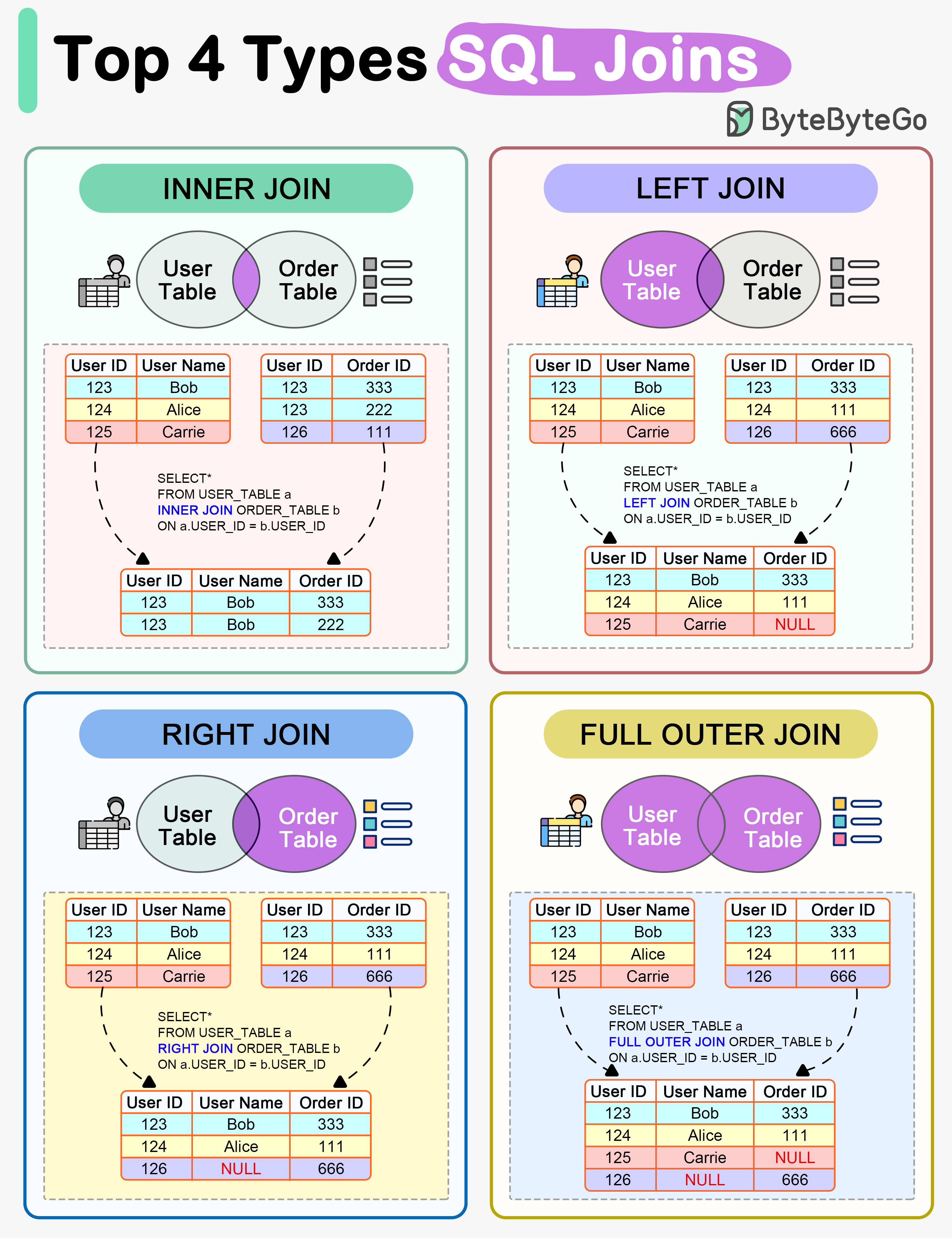
Join Type	Purpose	Example
`INNER JOIN`	Matching rows	`SELECT * FROM a JOIN b ON a.id=b.id;`
`LEFT JOIN`	All left rows	`SELECT * FROM a LEFT JOIN b ON a.id=b.id;`
`RIGHT JOIN`	All right rows	`SELECT * FROM a RIGHT JOIN b ON a.id=b.id;`
`FULL JOIN`	All rows	`SELECT * FROM a FULL JOIN b ON a.id=b.id;`
`CROSS JOIN`	Cartesian product	`SELECT * FROM a CROSS JOIN b;`

Constraint	Purpose
`PRIMARY KEY`	Unique row identifier
`FOREIGN KEY`	Reference another table
`UNIQUE`	No duplicate values
`NOT NULL`	Mandatory value
`CHECK`	Custom condition
`DEFAULT`	Default value

Indexes

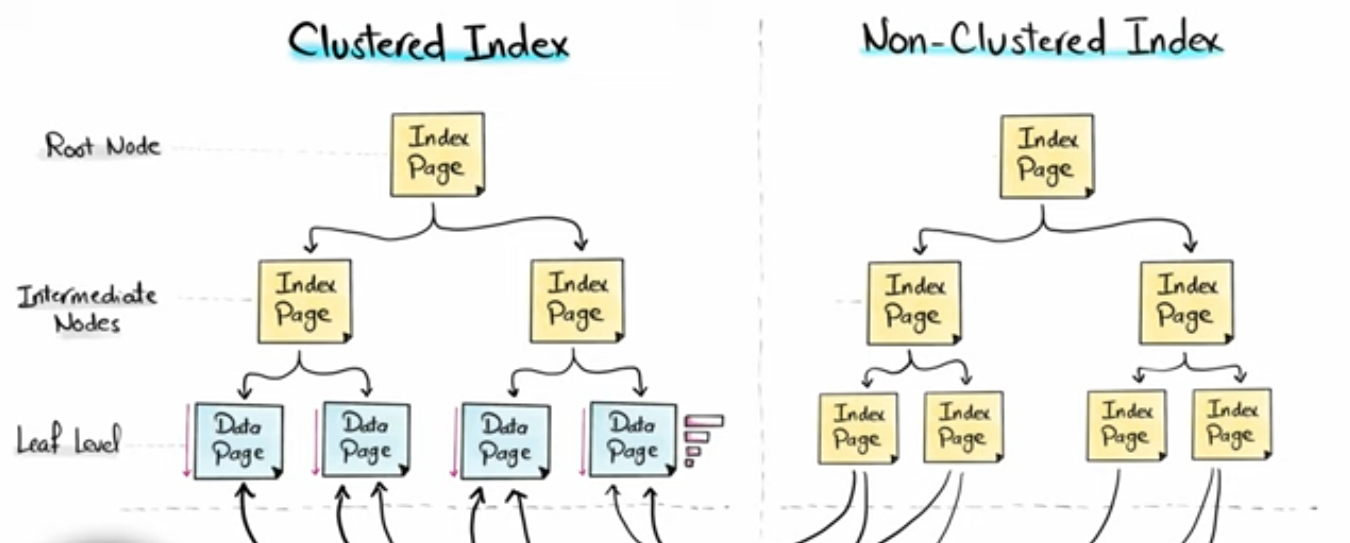
The smallest thing MSSQL reads from disk

One page = 8 KB

Think of a page like this:

+------------------------+
| Page Header            |
+------------------------+
| Row 1                  |
| Row 2                  |
| Row 3                  |
| ...                    |
+------------------------+
| Free Space             |
+------------------------+

Important rules:

MSSQL never reads half a page
If a row is on a page, the whole page comes into memory
Pages are addressed as (FileID, PageID)

Heap Table (NO Clustered Index)

A heap is the simplest possible storage.

CREATE TABLE Users (
  id INT,
  email VARCHAR(100),
  status VARCHAR(10)
);

No clustered index.

Physical reality on disk

Page 100:  (random order)
  (id=7, email=a@x, status=active)
  (id=2, email=b@y, status=inactive)

Page 205:
  (id=91, email=c@z, status=active)

Page 333:
  (id=15, email=d@q, status=active)

Key facts:

Rows are wherever space was available
No ordering
New rows go into any page with space
MSSQL tracks rows by RID = (FileID, PageID, SlotID)

To find a row:

MSSQL must know the RID
Otherwise → scan every page

Now add an index:

CREATE NONCLUSTERED INDEX idx_status ON Users(status);

Physical structure

Non-Clustered Index (B-tree):
  status='active' → RID (100, 3)
  status='active' → RID (333, 1)
  status='inactive' → RID (100, 2)

Query:

SELECT email FROM Users WHERE status='active';

What MSSQL does:

Traverse index → get RIDs
For each RID:
- Jump to that page
- Read entire page
Extract row

If rows are scattered:

Lots of random page reads
Cache-unfriendly
Slow at scale

Clustered Index Table

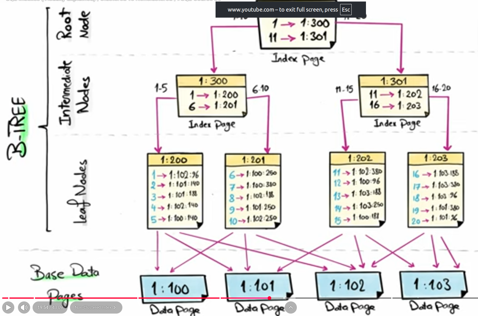
A table can have only one clustered index because the table’s rows can be physically ordered in only one way on disk.

Now recreate the table with a clustered index.

CREATE CLUSTERED INDEX idx_users_id ON Users(id);

This physically rewrites the table

Rows are now stored sorted by id.

Disk layout

Page 10 (leaf):
  id=1 | email=a@x | status=active | created_at=...
  id=2 | email=b@y | status=inactive | created_at=...

Page 11 (leaf):
  id=3 | email=c@z | status=active | created_at=...

Page 12 (leaf):
  id=4 | email=d@q | status=active | created_at=...

There is no separate table storage.

The leaf level of the clustered index IS the data pages

This is the most important sentence in MSSQL.

How MSSQL finds rows now

No RIDs
Rows identified by clustered key (id)

To find id = 7:

Traverse clustered B-tree
Land directly on Page 12
Row already there

One logical structure, one physical path.

Covered index

CREATE NONCLUSTERED INDEX idx_example ON Orders (customer_id, created_at) INCLUDE (total_amount, status);

which is similar to mongodb

db.Orders.createIndex({ customer_id: 1, created_at: 1 })

But total_amount and status are added to index but not used as for filter only for projection

How the index will be

Branch Nodes (Navigation):
- These only contain customer_id and created_at.
- They are sorted. This allows the engine to do a binary-style search (Index Seek) to find a specific customer or date range.
Leaf Nodes (The Final Results):
- These contain all four columns: customer_id, created_at, total_amount, and status.
- They also contain a pointer (the Row ID or Clustered Key) back to the original table.

when we query

SELECT total_amount, status 
FROM Orders 
WHERE customer_id = 5;

In this scenario, the database engine performs an Index-Only Scan (or Seek). It gets the answer directly from the index and never touches the actual table row

Index rules

MongoDB analogy

Compound index {a:1, b:1} supports:

{a}
{a, b}

But not {b} alone.

MYSQL

INDEX (A, B, C)

Supports:

A = ?
A = ? AND B = ?
A = ? AND B = ? AND C = ?
A BETWEEN x AND y

Does NOT support:

B = ?
C = ?
B = ? AND C = ?

If the first column isn’t used, the index is effectively invisible.

Rule (burn this in): Equality columns first, range columns last

SELECT total_amount
FROM Orders
WHERE customer_id = ?
  AND status = 'paid'
  AND created_at >= ?
ORDER BY created_at DESC;
 
//correct index
(customer_id, status, created_at)
 
wrong
(created_at, customer_id, status)

Once a range is hit, ordering breaks
Everything after becomes a scan

MongoDB has the same rule MSSQL just enforces it harder.

RULE

Equality filters: customer_id, status
Range filter: created_at
Select: total_amount
Order by: created_at

Why MSSQL Ignores Your Index (Real Reasons) Common causes:

Bad column order
Low selectivity (e.g., status)
Outdated statistics
Parameter sniffing
Query returns large % of table
Implicit conversions
Index too wide (IO cost

Statistics (The Brain Behind the Optimizer)

Before SQL Server chooses:

seek vs scan
index A vs index B
nested loop vs hash join

it must answer one question:

“How many rows will this operation produce?”

Everything else depends on that estimate. This is called cardinality estimation.

Suppose SQL Server estimates:

10 rows → nested loop is cheap
1,000,000 rows → nested loop is disastrous

Same query. Different estimates → different physical plan.

What a Statistic Actually Contains

Orders table with 1,000 rows. We have a column called Price.

the Price values in your table look like this:

500 rows are $10
200 rows are between $11 an d$ 99
250 rows are $100
50 rows are between $101 an d$ 500

The Header (The “Status Report”)

This tells the database how old the map is.

Updated: Jan 25, 2026
Rows: 1,000
Rows Sampled: 1000 (It looked at everything)

The Density Vector (The “Uniqueness”)

This is a single decimal number.

Density: 0.005
What it means: “On average, each price appears multiple times. It’s not a unique ID.”

The Histogram (The “Map”)

This is the most important part. SQL Server divides your data into “Steps” (buckets). Even if you have millions of rows, it uses a maximum of 200 steps to save space.

For our data, the Histogram would look like this simplified table:

Range High Key (The “Wall”)	EQ_ROWS (Exactly this value)	RANGE_ROWS (Values between this and previous)	AVG_RANGE_ROWS (Average count in between)
$10	500	0	0
$100	250	200	2.2
$500	5	45	1.1

How the Database uses this “Map”

Scenario A: You run SELECT * FROM Orders WHERE Price = 10

SQL looks at the Histogram.
It sees EQ_ROWS for $10 is 500.
The Decision: “500 rows is a lot! I’ll do a Table Scan because it’s more efficient than jumping back and forth with an index.”

Scenario B: You run SELECT * FROM Orders WHERE Price = 500

The “Ascending Key” Problem

Classic production bug. Example: WHERE created_at >= GETDATE() - 1

Stats histogram:

Built on old values
New values all look the same to optimizer

SQL Server assumes:

“Probably very few rows”

Reality:

Could be millions

Result:

Nested loops
Key lookups
Timeouts

This happens constantly on time-based tables.

Compression Strategy: SQL Server uses a “maximum difference” algorithm to choose which values become boundaries for these 200 steps. It looks for big “gaps” or spikes in your data to make sure the most significant values (like common prices or dates) get their own step.

NOTE: SQL Server does not automatically create a histogram for every column in your table because that would be a waste of resources. Instead, it creates them “on demand” or based on your indexes:

Index Statistics: When you create an index, a statistics object is automatically created. However, for a multi-column index (e.g., INDEX (City, State, Zip)), the histogram is only created for the first column (City). The other columns only get a “Density Vector” (a single number representing how unique they are).
Auto-Created Statistics: If AUTO_CREATE_STATISTICS is ON (the default), SQL Server will create single-column statistics the first time you use a column in a WHERE or JOIN clause, even if there is no index on it.
Manual Statistics: You can manually create statistics on any column or set of columns using the CREATE STATISTICS command.

Execution Plans

There are two different plans:

Estimated Execution Plan
- Built at compile time
- Based on statistics
- Shows optimizer assumptions
Actual Execution Plan
- Captured after execution
- Shows real row counts
- Reveals lies and mismatches

to see the plan

SET SHOWPLAN_ALL ON

Storage

Row Storage (MySQL default)

MySQL (InnoDB) is a row-store database.

That means:

Row = [col1, col2, col3, col4]

On disk:

Row1 → A B C D Row2 → A B C D Row3 → A B C D

Why row storage?

Optimized for:

OLTP
Single-row lookups
Inserts & updates

Indexes store column values, but the table itself is row-based.

Stored Procedures

Better Performance:

Pre-compilation: They are compiled once and their “execution plan” is cached. This means the database doesn’t have to re-parse the query every time it runs, making it faster for repeated tasks.
Reduced Network Traffic: Instead of sending a massive query over the network, your app just sends the name of the procedure and any parameters (e.g., EXEC GetUserOrders 101). This is a huge win for complex operations.

Enhanced Security:

Access Control: You can give a user permission to run a specific stored procedure without giving them access to the underlying tables. This prevents users from running “rogue” queries directly on your data.
SQL Injection Protection: Because they use parameters, they naturally separate the “code” from the “data,” making it much harder for attackers to inject malicious commands.

Centralized Business Logic:

One Source of Truth: If you have multiple apps (e.g., a web app, a mobile app, and a reporting tool) all using the same database, putting the logic in a stored procedure ensures they all calculate things (like tax or discounts) exactly the same way.
Easier Maintenance: You can fix a bug or change a calculation inside the database without having to re-deploy your entire application.

This is the #1 cause of slow stored procedures.

The Issue: When a procedure runs for the first time, SQL Server “sniffs” the input parameters and creates a specialized execution plan optimized for those specific values.

Why it’s slow: If the first user asks for a tiny amount of data (a “mouse”), SQL creates a fast plan for small results. If the next user asks for millions of rows (an “elephant”), SQL tries to use that same “small data” plan, which can be disastrously slow for a large dataset.

Parameter Sniffing (You Will See This)

Scenario: WHERE user_id = @user_id

First execution:

@user_id = 1 → 1 row
Plan optimized for 1 row it will be stored on cache

Second execution:

@user_id = 9000000 → 200k rows
Same cached plan reused
Disaster

When Parameter Sniffing Breaks Down

It fails when:

Data distribution is skewed
One parameter value represents 0.01% of rows
Another represents 50% of rows

Example:

@user_id = 1 — admin user, millions of rows @user_id = 900000 — normal user, 5 rows`

One cached plan cannot be optimal for both.

This is not a stored procedure problem it’s a data distribution problem.

Transcation

Below are clean, structured study notes distilled from your content.
No fluff, no metaphors, no emojis — only core concepts, mechanisms, and takeaways.

SQL Server Execution Plan — Study Notes

1. Why Execution Plans Exist

SQL queries can be executed in multiple ways.
The SQL Server Query Optimizer chooses a plan that it estimates to be the cheapest based on:
- Table size
- Indexes
- Statistics
- Available join strategies
The execution plan shows how SQL Server decided to execute a query step by step.

Purpose:

Identify performance bottlenecks
Decide where and which indexes to create
Validate whether indexes are actually used

2. Query Lifecycle (High Level)

SQL Server parses the query
Optimizer generates an execution plan
Plan is executed (data read, joined, aggregated)
Execution plan is cached for reuse
Same or similar query may reuse cached plan

3. Execution Plan Types

3.1 Estimated Execution Plan

Generated without executing the query
Based purely on statistics
Used to predict behavior
May differ from actual execution

3.2 Actual Execution Plan

Generated after query execution
Shows the real operators used
Includes actual row counts
Primary tool for tuning

3.3 Live Query Statistics

Shows execution progress in real time
Useful for long-running queries

4. Reading an Execution Plan

4.1 Direction

Read right → left
Data flows from rightmost operator to leftmost

4.2 Operators

Each icon represents an operation (scan, seek, join, sort, aggregate)
Arrow thickness indicates data volume

5. Table Structures

5.1 Heap

Table with no clustered index
Data stored unordered
Reads require Table Scan

5.2 Clustered Index

Data stored in B-tree structure
Physically ordered by clustered key
Reads use Clustered Index Scan or Seek

6. Scan vs Seek

6.1 Table Scan

Reads entire heap table
Worst access method
High I/O and CPU cost

6.2 Index Scan

Scans entire index or large portion
Better than table scan, still expensive

6.3 Index Seek

Navigates index directly to matching rows
Best access method
Minimal I/O

Priority (worst → best):

Table Scan → Index Scan → Index Seek

7. Execution Plan Properties (Key Metrics)

Actual Rows vs Estimated Rows
CPU Cost
I/O Cost
Physical Operator
Logical Operator
Index Used

Mismatch between estimated and actual rows:

Indicates outdated statistics or poor indexing

8. Sorting Behavior

Heap + ORDER BY

Requires explicit Sort operator
Additional CPU and memory cost

Clustered Index + ORDER BY (on key)

No sort required
Data already ordered

Benefit:

Clustered index eliminates runtime sorting

9. Nonclustered Index Usage

Scenario

Filtering on a non-key column

Before index:

Table Scan
Reads all rows

After nonclustered index:

Index Seek
Reads only matching rows

10. Key Lookup

Why It Happens

Nonclustered index contains only indexed columns
SELECT * needs additional columns
SQL Server fetches missing columns from clustered index

Behavior

Happens per matching row
Acceptable for small result sets
Expensive for large result sets

How to Eliminate

Select only indexed columns
Or use covering index (INCLUDE columns)

11. Join Algorithms

Nested Loops

Best for small input sets
Poor for large datasets

Hash Join

Best for large unsorted inputs
Uses memory and hashing

Merge Join

Best when both inputs are sorted
Efficient for large datasets

Optimizer chooses join based on:

Input size
Sort order
Available indexes

12. Aggregations on Large Tables

Rowstore (Clustered Index)

Reads many rows
High CPU and I/O
Costly for analytics

Columnstore Index

Column-based storage
Reads only required columns
High compression
Vectorized execution