
Types
Encoder-only
These models convert an input sequence of text into a rich numerical representa‐ tion that is well suited for tasks like text classification or named entity recogni‐ tion. BERT and its variants, like RoBERTa and DistilBERT, belong to this class of architectures.
Decoder-only
Given a prompt of text like “Thanks for lunch, I had a…” these models will auto- complete the sequence by iteratively predicting the most probable next word. The family of GPT models belong to this class.
Encoder-decoder
These are used for modeling complex mappings from one sequence of text to another; they’re suitable for machine translation and summarization tasks. In addition to the Transformer architecture, which as we’ve seen combines an encoder and a decoder, the BART and T5 models belong to this class.
- query — asking for information
- key — saying that it has some information
- value — giving the information
Encode help us to understand the text very well so it can be used for classification other thing realted to text that we have.
Mixture of Experts (MoE) Architecture
In MoE models, not all parts of the model are active at once. Instead, a small subset of “experts” (different sub-models or layers) are selected to process each input. This helps with scalability and efficiency by allowing the model to scale without significantly increasing computational costs.
- How it works: At each step, a gating mechanism chooses which experts (sub-models) will be active for a particular input. Only a few experts are used for each forward pass, making the model more efficient by reducing the number of active parameters.
- Key idea: Selective computation by activating only a subset of experts for a given input.
- Example models: Switch Transformer, GShard, and MoE-based models like the ones used by Google.
State Space Models (SSM)
State Space Models are designed to handle sequential data in a more efficient manner, improving memory usage and scaling to longer sequences. SSMs are an alternative to the standard transformer architecture and are particularly useful for tasks involving long-range dependencies in data.
-
How it works: SSMs use continuous latent states to capture sequential dependencies, while transformers typically use discrete tokens. The architecture combines the benefits of both recurrent neural networks (RNNs) and transformers by treating the sequence as a set of continuous latent variables that evolve over time.
-
Key idea: Improve memory efficiency and scale better for long-range dependencies in sequences.
-
Example models: Linear Transformers, Reformer, and Longformer (which also uses sparse attention mechanisms).
Transformer Top to bottom
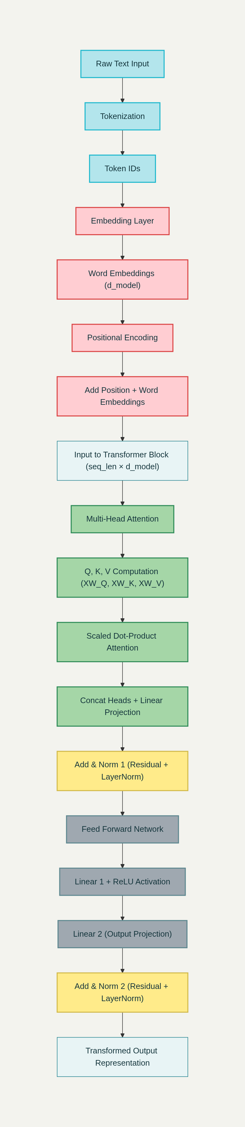
A transformer contain both encoder and decoder where encoder is used to convert the given text in to meaningfull vectors.
Decoder use the self attention vectors and predict the next word
First the input is converted to tokens for each word we have vocobalry map where the word will be converted to
Every tokenizer builds a vocabulary: a dictionary mapping each token string to an integer ID.
Some common tokenizer are
- Byte Pair Encoding (BPE) remains the dominant tokenization method Refer
- Adaptive Tokenization
- Boundless BPE

Token IDs are converted to dense vector representations through an embedding layer:
-
Embedding dimension: Typically 512, 768, 1024, or higher in large models
-
Learnable parameters: Each token has a corresponding embedding vector
-
Semantic encoding: Similar words have similar embedding vectors in high-dimensional spac
-
A token ID like
15496is just a number. -
But to feed it into a neural network, we need a vector a list of real numbers that captures the token’s meaning and context.
-
This is what the embedding layer does: it maps token IDs → vectors.
Example
"Hello world"

   ↓tokenization

[15496 ,995]

   ↓ Embedding

[
  [0.017, -0.038, ..., 0.204],   # Embedding vector for "Hello"
  [-0.085, 0.124, ..., 0.056]    # Embedding vector for " world"
]
- Each number represend the meaning of hello to his feature vector it has
Open Source Embedding models
Two key resources for open-source embeddings:
- Sentence Transformers (expert.net): This Python framework simplifies loading and using various embedding models, including the popular “all-mpnet-base-v2” and “all-MiniLM-L6-v2”.
- Hugging Face (huggingface.co): This platform hosts a vast collection of machine learning models and datasets, including the “Massive Text Embedding Benchmark” (MTEB) project, which ranks and evaluates embedding models.
Choosing the Right Embedding Model
- Task: Different models specialize in different tasks, like semantic search, clustering, or bitext mining.
- Performance: The MTEB leaderboard offers a valuable resource for comparing model performance across various tasks.
- Dimension Size: Smaller dimensions generally result in faster computation and lower memory requirements, especially for similarity searches.
- Sequence Length: Models have limitations on the input length (measured in tokens), impacting how you process longer documents.
Optimizing Embedding Generation
-
Mean Pooling: This aggregation method combines multiple embeddings into a single representative embedding, essential for sentence-level comparisons.
Example: Text embedding model will return text the probablity of passed text with the no of vocabulary it has let say we have a text embedding model with dimension of 468 then it have 468 voc so it will return the probablity of passed text with all 468 word but if we want a single probablity we need to use meanpooling
-
Normalization: Normalizing embeddings (creating unit vectors) enables accurate comparisons using methods like dot product.
-
Quantization: This technique reduces the precision of model weights, shrinking the model size and potentially improving inference speed.
-
Caching: Transformers.js automatically caches models in the browser, significantly speeding up subsequent inference operations.
For more Vector DB and embedding
Position encoding
Transformers process a sentence as a bag of tokens (parallel) no natural sense of order.
But language has order:
- “dog bites man” ≠ “man bites dog”
So we add positional information to word embeddings → the model knows token order
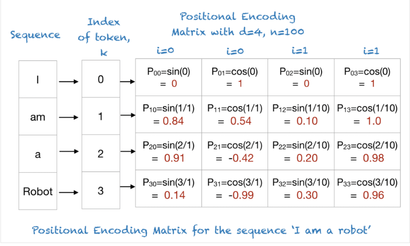
For each position (0,1,2,…) and each embedding dimension :
- = token’s index in the sequence (0th, 1st, 2nd …).
- = embedding dimension (e.g., 512).
- = dimension index (0, 1, 2 …).
- Even indices → sine; odd indices → cosine.
So each position gets a vector of size .
Let’s say:
- Sentence:
"I love AI" - Word embeddings dimension (to keep it tiny).
Step 1: Positions
"I"→ position 0"love"→ position 1"AI"→ position 2
Step 2: Apply formula
For position 1, with :
So the positional vector for "love" is:
Add to Word Embedding
Suppose the embedding for "love" was:
We add position encoding element-wise:
Now the model knows both the meaning (“love”) and where it occurs (position 1).
Why that formula ?
What we want from positional encodings
When we add positional encodings to word embeddings, we want them to have these properties:
- Every position is unique → word at position 5 should not look like word at position 50.
- Relative distances should be meaningful → the difference between encodings of position 5 and 6 should have the same “shape” as between 50 and 51.
- Work in any sequence length → no matter if sequence is 10 words or 1000.
- Encodings should smoothly vary → so nearby positions have nearby encodings.
Why not just sin(pos) or cos(pos)?
- If we did only
sin(pos): - At
pos=0,sin(0)=0. - At
pos=π,sin(pos)=0again. - That means different positions can look identical → bad for uniqueness.
So plain sin (or plain cos) would repeat every 2π, which destroys the ability to tell apart positions beyond that range.
Why both sin and cos?
-
Using both ensures we can distinguish shifts. Example:
-
sin(θ)andcos(θ)together form a 2D vector (like coordinates on a circle). -
This way, each position maps to a unique point on a spiral curve across dimensions.
-
Also, later layers can compute relative positions easily using linear operations (since sine and cosine preserve phase differences).
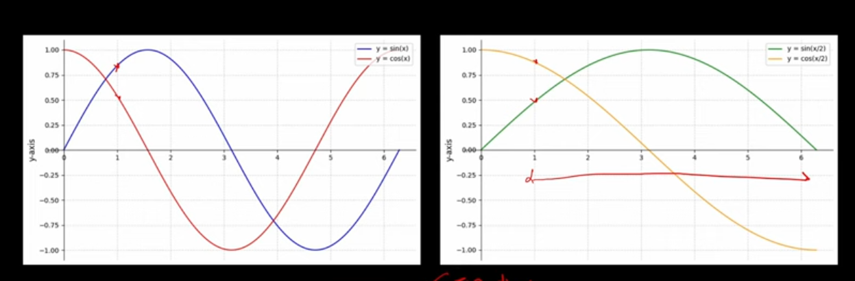
So we taking sin and cos in differerent frequency such that no two vector will have same postion encoding
A visluation on each

Why not simple numbers (1,2,3,…) fail
Let’s think about what properties we want from a position encoding.
- Uniqueness – every position has a unique code.
- Continuity – nearby positions should have similar encodings.
- Relative meaning – the model should be able to infer “how far apart” two tokens are.
- Generalization – the model should handle sequences longer than it was trained on. Now check the linear indices:
- (1,2,3) → unique (ok)
- distances: (2−1)=1, (3−1)=2 — yes, numeric distance encodes relative position (ok)
- but dot products grow unbounded with higher numbers (no)
- and the model can’t generalize to unseen positions (e.g. position 512 if trained on 1–100) (no)
Reason: A linear embedding like 100 vs 101 are numerically close, but in the vector space, those large scalar values distort similarity measures used in attention (dot products). The model cannot easily learn position differences in a stable way.
Instead of absolute integers, we want an encoding that:
- stays bounded (so scaling doesn’t explode),
- encodes relative distances in its structure,
- and has a smooth gradient so the model can interpolate between known positions.
Encoder
Where feed forward network is the learning happens like how we did on multilayer preceptron or sequential model the feed forward layer will learn the pattern the self attention layer helps to find and detect attention to the words
Self -Attention
The self-attention mechanism involves three main components:
- Query (Q): The query is the token that is being processed.
- Key (K): The key is the token to which we are checking compatibility with the query.
- Value (V): The value is the actual representation vector of the token.
For each word embedding we create a Query vector, a Key vector, and a Value vector. These new vectors are smaller in dimension than the embedding vector. Their dimensionality is 64, while the embedding and encoder input/output vectors have dimensionality of 512.
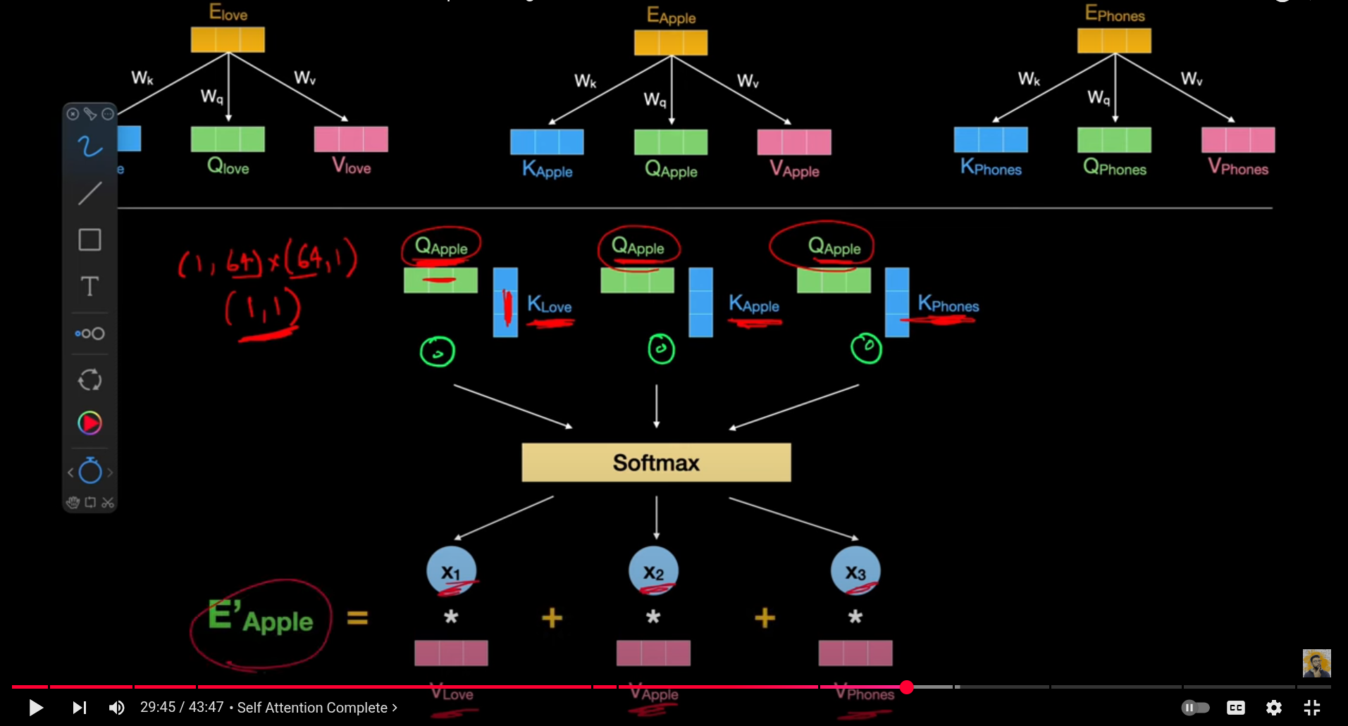
We will have Wq,Wk,Wv for all input and we multiply the input embedding with that we get Q,K,V
input X * Wq , X * wk , X * wv ⇒ which give query
Now to compute attention we multiply each Q with other K vector then divde that vaule by root of dimension of K vector to stablize the gradient
Next apply softmax to our vector we have and multiply with vaule vctor of each corresponding
Single formula for repersentating above
Attention(Q, K, V) = softmax(Q * K^T / sqrt(d)) * V
where:
Qis the query vectorKis the key vectorVis the value vectordis the dimensionality of the key vector^Tdenotes the transpose operationsoftmaxis the softmax function*denotes the matrix multiplication operation
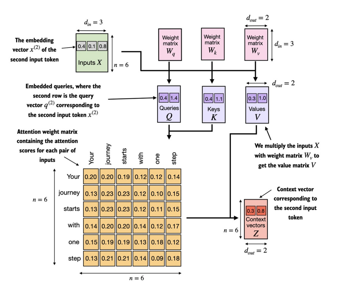
- Each word in the input sequence is embedded into a vector space using a learned embedding matrix.
- For each word, three vectors are computed:
Q,K, andV. These vectors are computed by applying three separate linear transformations to the word’s embedding vector. - The
Qvector is used as a query to compute attention weights with respect to all other words in the sequence. This is done by taking the dot product of theQvector with theKvectors of all other words, and applying a softmax function to obtain a set of attention weights. - The attention weights are then used to compute a weighted sum of the
Vvectors of all other words, which produces the output of the self-attention mechanism.
Multi head attention
Single attention layer cannot detect all attention on the sentence when it grows so we use multihead attention where we have mutli attention layer and each will foucus on specific thing
Dont think that multi head attention is computation costly
- Instead of doing one big attention with large dimension
d_model, - We split it into h smaller attentions (heads), each of size
d_model/h. - Then we run attention in parallel and combine results.
Suppose:
- Sequence length =
n = 4tokens - Embedding size =
d_model = 8So: Q, K, Veach have shape[n × d_model] = [4 × 8]. When we compute attention scores:
That is [4×8] × [8×4] = [4×4] (the attention score matrix).
Cost ≈ n² × d_model = 4² × 8 = 128 operations
MultiHead
Now instead of 1 big head (dimension 8),
we split into 2 heads, each of size d_model/h = 8/2 = 4.
So for each head:
-
Q_i, K_i, V_ieach have shape[4 × 4]. -
Compute
Q_i K_i^T:[4×4] × [4×4] = [4×4].
Cost per head ≈ n² × (d_model/h) = 16 × 4 = 64
We have 2 heads, so total cost = 64 + 64 = 128.
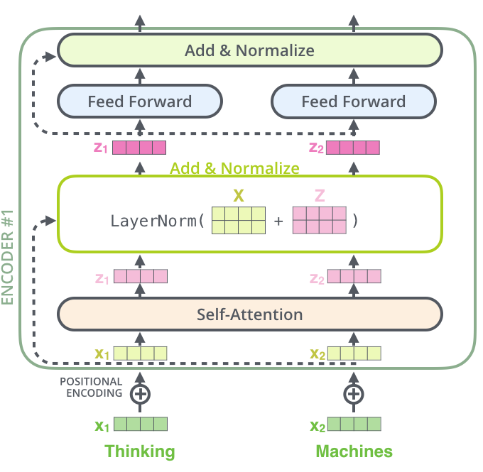
Normalization
Neural networks sometimes produce values that are too large, too small, or unstable across different layers. This makes training harder because gradients (updates) can either explode or vanish.
The idea of normalization:
- Look at the numbers in one vector (say a token’s representation:
[2.4, -1.7, 0.5, 3.1]). - Compute their mean (average).
- Compute their standard deviation (spread).
- Rescale them so that the new vector has mean ≈ 0 and std ≈ 1.
Then we add two learnable numbers ((\gamma, \beta)) so the model can still stretch/shift if needed.
Why it helps:
- Keeps all features at a similar scale.
- Prevents “one feature dominates” problems.
- Stabilizes training → gradients behave nicely.
Think of it like re-centering and re-scaling your data every step so the network always works in a healthy range.
Feed-Forward Network (FFN)
Attention mixes information between tokens (e.g., “cat” attends to “sat”),
but each token also needs extra processing on its own to detect patterns like “is this a verb?” or “is this sentiment positive?”
in here only actual learning is happen model learn to detect patterns.
Each token vector goes through a little mini neural network, separately, position by position:
- Multiply by a big weight matrix (W_1) → expand dimensions (make it fatter).
- Apply a non-linear function (ReLU, GELU, etc.) → adds complexity.
- Multiply by another matrix (W_2) → shrink back to original size.
-
Gives non-linear transformations (attention alone is linear).
-
Lets each token build more abstract features.
-
Most parameters in transformers actually live in the FFN (it’s the “heavy lifting” part).
-
Attention = “Who should I listen to?”
-
FFN = “Now that I’ve listened, how do I transform this info into a stronger feature?”
Decoder
 The encoder takes the input sequence (like a sentence in French) and turns it into a set of context-rich vectors.
The decoder takes those vectors and generates the output sequence step by step (like an English translation).
So:
- Encoder → encodes meaning/context of the input
- Decoder → turns that meaning into output tokens, one at a time
Language is sequential:
- To predict the next word, you need to know the words already generated.
- Example: If we already generated
"I am", the next likely token could be"happy","hungry", etc. - But we should not peek into the future words that haven’t been generated yet. That’s why decoders generate autoregressively → one token at a time.
If we trained the decoder by literally generating one token at a time, it would be very slow.
Imagine a 100-word sentence → you’d have to do 100 forward passes just for one training example.
Instead, we want to train all positions in parallel (so GPUs can batch them).
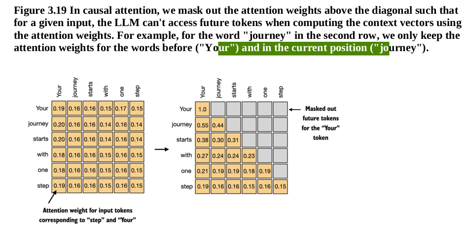
Solution: Masked Self-Attention
- Use the whole target sentence as input during training (not just past tokens).
- But apply a mask so each position can only “see” past tokens, not future ones.
Example target sentence:
I am happy today
- Position 1 (
I) → sees onlyI - Position 2 (
am) → seesI, am - Position 3 (
happy) → seesI, am, happy - Position 4 (
today) → seesI, am, happy, today
So the model is still learning to predict one token at a time, but it’s done in parallel with masking.
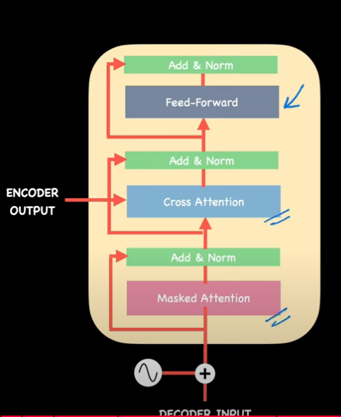
The decoder block has two attentions + FFN:
- Masked Self-Attention
- Lets decoder look at already-generated tokens (but not future ones).
- Encoder–Decoder Attention
- Lets decoder look at the encoder’s output (the source sentence’s meaning).
- Feed-Forward Network + Norm
- Same as encoder: transformation + stabilization.
Optimizer and loss Self attes function
Optimizer: The optimizer in a Transformer model refers to the algorithm used to update the model parameters during training in order to minimize the loss function. Some common optimizers used in Transformer models include:
-
Adam (Adaptive Moment Estimation): This is a popular optimizer that computes adaptive learning rates for each parameter. It combines the advantages of two other extensions of stochastic gradient descent, namely AdaGrad and RMSProp.
-
AdamW: This is a variant of Adam that incorporates weight decay regularization directly into the optimizer, which can stabilize training and improve generalization.
-
SGD (Stochastic Gradient Descent): Though less commonly used in Transformers compared to Adam variants, SGD updates model parameters based on the gradient of the loss function with respect to the parameters.
-
AdaGrad and RMSProp: These are older optimizers that adjust the learning rates of model parameters based on the frequency of their updates during training.
NOTE (my understanding): When training a deep learning model, we repeatedly feed training data and compute the loss. Using backpropagation, we get gradients that show how each weight affects the loss. The optimizer (like SGD or Adam) then updates the weights in the right direction and magnitude to minimize the loss. Over many updates, the optimizer helps the model gradually find a set of weights that produce good predictions.
| Concept | Role |
|---|---|
| Loss function | Measures how wrong predictions are |
| Gradients | Tell how to adjust each weight |
| Optimizer | Applies a rule for how fast and in what way to adjust weights |
| Training loop | Repeats this process over data until loss stops improving |
Casual Attention mechanism
Causal attention is a variant of attention mechanism, commonly used in natural language processing, especially in autoregressive models like GPT and Transformer-based models for tasks like language generation. The term “causal” refers to the property that the attention mechanism ensures that the model only attends to past tokens when predicting the next token. This is essential for autoregressive models, which generate tokens sequentially, one at a time, and should not “look ahead” into future tokens.
While causal attention has benefits in sequence generation, it comes at the cost of reduced parallelism during training, especially when compared to bidirectional attention models like BERT, where all tokens attend to each other.
SGD
Batch Gradient Descent: Computes the gradient of the loss function with respect to the parameters for the entire training dataset and updates the parameters once per iteration. This can be computationally expensive for large datasets.
Stochastic Gradient Descent: Computes the gradient of the loss function for each training example individually and updates the parameters for each training example. This makes SGD much faster and more efficient for large datasets.
Logits
Logits are the raw, unnormalized scores or outputs from a machine learning model, often used in classification tasks. In simpler terms, logits represent the values produced by a neural network before applying an activation function like softmax or sigmoid, which converts these raw values into probabilities.
How it used in GPT
- After tokenization, the tokens are passed through the model (like GPT). The model is a neural network that predicts the next token in the sequence based on the previous ones.
- The model outputs logits for each possible token in its vocabulary. If the model has a vocabulary of 50,000 tokens, it will produce 50,000 logits as raw scores for each token after processing the current input sequence.
- The logits are then passed through a softmax function to convert them into a probability distribution over the vocabulary. The softmax function transforms the logits into probabilities that sum to 1, which indicates how likely each token is to follow the current sequence.
BERT Model
has 768 feature vector for embedding and BERT has a fixed vocabulary of 30,000 words (or tokens).
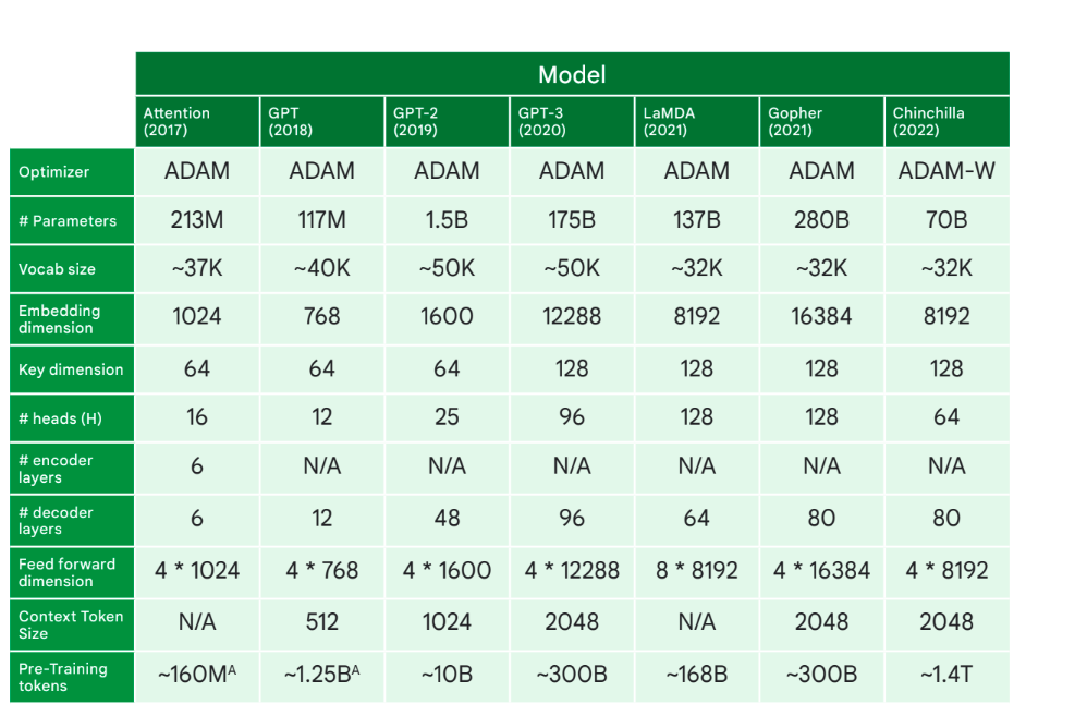
GPT-3 has 50,257 words of voc and 12288 dimension
query,key have 128 * 12,288 dimension
vaule = 12288 * 12288
96 head attention
Has 12 layer of encoder only
Handling Unknown Words
- Subword Tokens: When BERT encounters a word that is not in its vocabulary, it uses the WordPiece tokenization to break it into subword units that are in the vocabulary. This means that even if a word is not directly known, its subcomponents likely are, allowing the model to still process and understand it.
- [UNK] Token: In cases where a word or subword cannot be tokenized into known vocabulary units, it is represented by a special token [UNK] (unknown). However, this is rare due to the effectiveness of the WordPiece tokenization
Embedding Representation
The maximum sentence length is 512 tokens.
Word Embeddings: Each token in the vocabulary is represented by a 768-dimensional vector (in the case of BERT-base). This means that after tokenization, each subword token is converted into its corresponding embedding.
Positional Embeddings: BERT also uses positional embeddings to encode the position of each token in the sequence, ensuring that the model can understand the order of words.
Segment Embeddings: If the input consists of multiple segments (e.g., a pair of sentences), segment embeddings are used to differentiate between them.
Transformer models, including BERT, require input sequences to be of the same length. Since text sequences can have varying lengths, shorter sequences are padded with a special token (usually [PAD]) to match the length of the longest sequence in the batch.
Vector masks help distinguish between actual data and padding. This ensures that the model does not treat padding tokens as meaningful input.
# Input: [101, 2054, 2003, 1996, 512, 0, 0, 0]
# Attention Mask: [1, 1, 1, 1, 1, 0, 0, 0]
Here, 101, 2054, 2003, 1996, 512 are real tokens, and the remaining are padding tokens.
BERT requires special tokens [CLS] at the beginning and [SEP] at the end of each input sequence. For sentence pairs, [SEP] is also used to separate the two sentences.
from transformers import BertTokenizer

# Initialize the tokenizer
tokenizer = BertTokenizer.from_pretrained('bert-base-uncased')

# Example sentences
sentence1 = "What is the capital of France?"
sentence2 = "Paris is the capital of France."

# Tokenize with padding and truncation
encoding = tokenizer(
    sentence1, sentence2,
    add_special_tokens=True,  # Add [CLS] and [SEP]
    max_length=20,  # Pad & truncate all sentences to 20 tokens
    padding='max_length',  # Pad to max_length
    truncation=True,  # Truncate to max_length
    return_tensors='pt'  # Return PyTorch tensors
)

# Print the encoded inputs
print("Input IDs:")
print(encoding['input_ids'])
print("\nAttention Mask:")
print(encoding['attention_mask'])
print("\nToken Type IDs:")
print(encoding['token_type_ids'])

for sent in sentences:
    # `encode` will:
    #   (1) Tokenize the sentence.
    #   (2) Prepend the `[CLS]` token to the start.
    #   (3) Append the `[SEP]` token to the end.
    #   (4) Map tokens to their IDs.
    encoded_sent = tokenizer.encode(
        sent,  # Sentence to encode.
        add_special_tokens=True,  # Add '[CLS]' and '[SEP]'
        # This function also supports truncation and conversion
        # to pytorch tensors, but we need to do padding, so we
        # can't use these features :( .
        # max_length = 128,          # Truncate all sentences.
        # return_tensors = 'pt',     # Return pytorch tensors.
    )
    print(encoded_sent)
Tokenization
Tokenization is the process of breaking down text into smaller units called tokens, which are then used as input for the LLM. Tokens can represent individual characters, words, or subwords.
Byte Pair Encoding (BPE):
Training: BPE starts with a large corpus of text and initially treats each character as a separate token. The algorithm then iteratively merges the most frequent pairs of tokens into new tokens. This process continues until a desired vocabulary size is reached.
Example: Byte Pair Encoding (BPE) is a simple form of data compression that replaces the most frequent pair of adjacent bytes in a sequence with a single byte. It’s often used in text processing, particularly in natural language processing tasks.
How Byte Pair Encoding Works
- Initialization: Start with a sequence of bytes (or characters).
- Counting Pairs: Count all adjacent pairs of bytes in the sequence.
- Replace the Most Frequent Pair: Identify the most frequent pair and replace it with a new byte (a byte that doesn’t exist in the original sequence).
- Repeat: Repeat the counting and replacing process until a certain condition is met (like a maximum number of replacements).
Example
Let’s say we have the following simple sequence of characters:
ABABABA
Step 1: Count Pairs
- The pairs are:
AB,BA,AB,BA,AB - Frequencies:
AB: 3 timesBA: 2 times
Step 2: Replace the Most Frequent Pair
- The most frequent pair is
AB. Let’s say we replaceABwithC(a new byte). - New sequence:
C C A
Step 3: Update and Repeat Now, we have the sequence:
C C A
- Pairs:
C C,C A - Frequencies:
C C: 1 timeC A: 1 time
No pair is more frequent than the others, so we stop here.
3. Pre-tokenizers:
- Function: Pre-tokenizers handle spaces and punctuation before applying the main tokenizer. They can optimize the tokenization process by treating spaces as boundaries, avoiding merging tokens across spaces.
4. Tokenization in Practice:
- Vocabulary Size: The number of unique tokens determines the output dimensionality of the language model.
- Handling New Tokens: LLMs generally do not handle new tokens well. Choosing a comprehensive tokenizer and vocabulary is critical.
- Choosing the Largest Token: When applying the tokenizer, the algorithm always selects the largest available token. For instance, it would prioritize “token” over “t” if both are present in the vocabulary.
- Computational Considerations: Tokenization has computational costs. Efficient algorithms and techniques are used to speed up the process.
- Future of Tokenizers: There’s debate about the necessity of complex tokenizers. Character-level or byte-level tokenization might become more prevalent as architectures evolve to handle longer sequences efficiently.
5. Challenges with Tokenization:
- Domain-Specific Tokenization: Specialized domains like math and code often require custom tokenization schemes.
- Impact on Evaluation: Perplexity, a common LLM evaluation metric, is sensitive to the choice of tokenizer, making comparisons between models difficult.
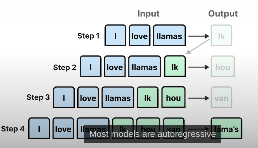
AutoRegressive
Let say we giving input as hi hello how LLM will predict next are once it predicted single word it will be append to input hi hell how are and again send to LLLM it will keep happens until end this type of models called autoregressive
KV cache
The Key-Value (KV) cache is a memory optimization technique used in transformer-based Large Language Models (LLMs) to speed up the generation of text. It stores previously computed key and value tensors from the attention layers, allowing the model to avoid redundant computations.
Transformers use the self-attention mechanism to decide which words in a sentence should influence each other. This mechanism operates as follows:
- Each token in the input is converted into three vectors:
- Query (Q) – What this token is looking for in others.
- Key (K) – How relevant this token is to queries.
- Value (V) – The actual information of this token.
- Self-attention computes similarity scores:
- Each token’s query (Q) is compared against the keys (K) of all previous tokens.
- The resulting attention scores determine how much focus each token should have on the others.
- Weighted sum of values:
- The values (V) are weighted according to the attention scores.
- The weighted values are summed to produce the next token.
- Each token requires storing two large tensors (K and V) per layer.
- For GPT-3 (175B parameters), storing KV cache for 2048 tokens can require hundreds of GBs.
- Existing models store KV contiguously, leading to memory fragmentation and waste.
LLM traning methods
Causal Language Modeling (CLM)
CLM is an autoregressive method where the model is trained to predict the next token in a sequence given the previous tokens. CLM is used in models like GPT-2 and GPT-3 and is well-suited for tasks such as text generation and summarization. However, CLM models have unidirectional context, meaning they only consider the past and not the future context when generating predictions.
Masked Language Modeling (MLM)
MLM is a training method used in models like BERT, where some tokens in the input sequence are masked, and the model learns to predict the masked tokens based on the surrounding context. MLM has the advantage of bidirectional context, allowing the model to consider both past and future tokens when making predictions. This approach is especially useful for tasks like text classification, sentiment analysis, and named entity recognition.
Sequence-to-Sequence (Seq2Seq)
Seq2Seq models consist of an encoder-decoder architecture, where the encoder processes the input sequence and the decoder generates the output sequence. This approach is commonly used in tasks like machine translation, summarization, and question-answering. Seq2Seq models can handle more complex tasks that involve input-output transformations, making them versatile for a wide range of NLP tasks.
Knowledge Distillation
This technique involves transferring knowledge from an LLM (teacher) to an SLM (student), enabling the smaller model to learn and mimic the capabilities of the larger one.
Knowledge distillation can be implemented in two ways:
-
White-box distillation: The student model has full access to the teacher model’s internal architecture and parameters (e.g., DistilBERT)
-
Black-box distillation: The student model only has access to the teacher model’s outputs, learning to replicate the teacher’s behavior without direct insight into its internal working
Model
A deep learning model is fundamentally two parts:
-
Structure
This is the computational graph — the blueprint that describes how inputs are transformed into outputs. In PyTorch, this is implemented as classes that subclasstorch.nn.Module. Layers likeLinear,Conv2d, orTransformerBlockare the building blocks. -
Parameters
These are the learned numerical values (weights and biases) that store the model’s “knowledge.” Parameters are represented astorch.nn.Parameterobjects, which are specializedtorch.Tensorinstances withrequires_grad=True. The parameter data must be stored in either system RAM or GPU VRAM, depending on where the computation happens.
A model = STRUCTURE + PARAMETERS
STRUCTURE:
- The recipe for computation (layers, ops, connections)
- PyTorch: nn.Module classes
- TensorFlow: tf.keras.Model or SavedModel
PARAMETERS:
- Learned numbers → weights & biases
- Actually stored floats (usually float32 → 4 bytes each)
- This is where “knowledge” lives
Example: Tiny Linear Model
class TinyModel(nn.Module):
	def __init__(self):
		super().__init__()
		self.linear = nn.Linear(2, 1)

model = TinyModel()
• STRUCTURE: Linear layer → y = Wx + b • PARAMETERS:
- W: shape [1, 2]
- b: shape [1]
In Memory:
• W = 2 floats → 8 bytes • b = 1 float → 4 bytes • Total tiny brain = 12 bytes!
Saved to File:
torch.save(model.state_dict(), "weights.pt")Saved dict:
{
'linear.weight': tensor([[...]]),
'linear.bias': tensor([...])
}
How Parameters Are Stored and Moved
In PyTorch, when you write model.to('cuda') or model.cuda(), the following occurs:
- PyTorch allocates memory on the GPU for each parameter tensor.
- It copies the numerical data from system RAM to GPU VRAM.
- The
Tensorobject’s internal storage pointer is updated to point to the new GPU buffer. - The computation graph itself stays in Python/C++ — only the data buffers move to the GPU.
If your model’s parameters do not fit into the available GPU VRAM, this operation fails with an out-of-memory error.
What Happens if the Model Is Larger than Available VRAM
Large models, such as those with tens of billions of parameters, cannot fit into the VRAM of a single consumer GPU. To run them, various techniques are used:
- Model Parallelism
The model’s parameters are split across multiple GPUs. Each GPU holds a slice of the full parameter set and processes only its part of the computation. GPUs exchange partial results during computation, typically using high-speed interconnects like NVLink or PCIe. - Offloading and Paging
Specialized frameworks keep parts of the model in system RAM or even on disk and load only the necessary chunks to the GPU at runtime. This is done layer by layer or block by block. Libraries like DeepSpeed, vLLM, and bitsandbytes implement such strategies for large language models. - Quantization
Instead of storing weights in 32-bit floating point (float32), they can be compressed to lower precision formats such as int8 or int4. This greatly reduces the memory footprint while sacrificing minimal accuracy, enabling much larger models to run on smaller GPUs. - Specialized Runtimes
In production, frameworks like Hugging Face Accelerate or inference engines like TensorRT or ONNX Runtime handle low-level optimizations, device placement, and memory management. Some can automatically handle sharding or offloading to improve efficiency.
VRAM Limits in Practice
If multiple inference requests run in parallel, VRAM usage can spike proportionally. This means one must control concurrency, use batch processing carefully, or fall back to CPU execution when the GPU is full. Running models with ONNX Runtime on CPU avoids VRAM limits but can be slower.
Resources
- Deconstructing BERT Part 2: Visualizing the Inner Workings of Attention
- Transformers: The Architecture
- BERTViz GitHub Repository
- A Gentle Introduction to Positional Encoding in Transformer Models (Check)
- Illustrated Transformer
- Transformers Explained
- Getting Started with PyTorch 2.0 Transformers
- Tutorial 14: Transformers I - Introduction
- BERT Notes
- The Effectiveness of Recurrent Neural Networks
- Llama3 from Scratch
- Finetuned Spam Classifier
- https://prvn.sh/the-animated-transformer/
- Ecco GitHub Repository
- The Transformers Architecture in Detail: What’s the Magic Behind LLMs
- https://rbcborealis.com/research-blogs/tutorial-14-transformers-i-introduction/
- How Do Language Models put Attention Weights over Long Context?
- Understanding LLMs from Scratch Using Middle School Math
- Orignal transformer paper “Attention is all you need” introduced by a layman | Shawn’s ML Notes
- https://learn.deeplearning.ai/courses/how-transformer-llms-work/lesson/nfshb/introduction
- https://github.com/tanishqkumar/beyond-nanogpt/tree/main
- made a transformer by hand (no training!)
- I made a transformer by hand (no training!)
- https://towardsdatascience.com/deep-dive-into-self-attention-by-hand-%EF%B8%8E-f02876e49857/
Visualizer
-
Transformer Explained Visually: Learn How LLM Transformer Models Work with Interactive Visualization
-
https://freedium.cfd/https://ai.gopubby.com/llms-do-not-predict-the-next-word-2b3fbe39900f
The Big LLM Architecture Comparison
- https://towardsdatascience.com/deep-dive-into-self-attention-by-hand-%EF%B8%8E-f02876e49857/
- https://cgnarendiran.github.io/blog/rope-is-attention-all-you-really-need/
- https://yaofu.notion.site/How-Do-Language-Models-put-Attention-Weights-over-Long-Context-10250219d5ce42e8b465087c383a034e