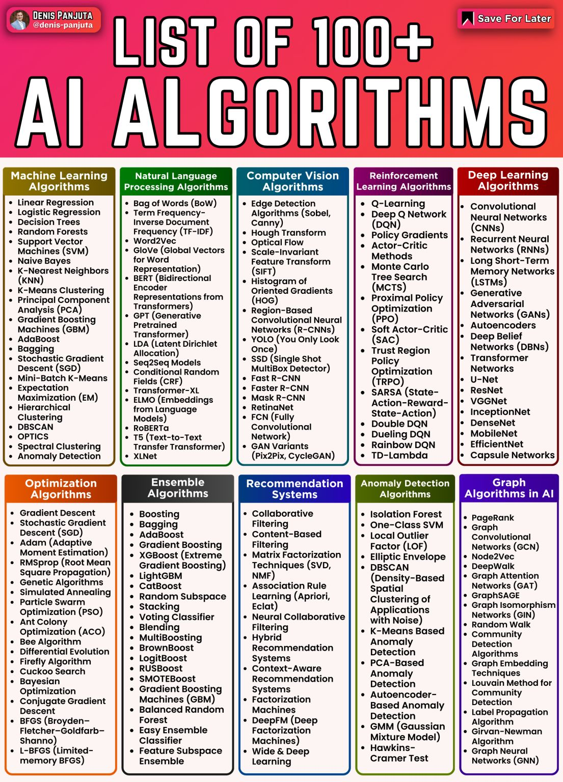
Machine learning

Machine learning

• Supervised learning → Train data with lables
• Unsupervised learning → FInd pattern in data and create a cluster
• Reinforcement learning →based on feedback

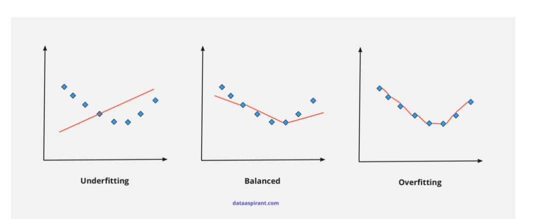
Generalization

Generalization in machine learning refers to the ability of a trained model to accurately make predictions on new, unseen data. The purpose of generalization is to equip the model to understand the patterns and relationships within its training data and apply them to previously unseen examples from within the same distribution as the training set. Generalization is foundational to the practical usefulness of machine learning and deep learning algorithms because it allows them to produce models that can make reliable predictions in real-world scenarios.

It should not perform good only to the test data or traning data it also need to perfrom well on unseen new data

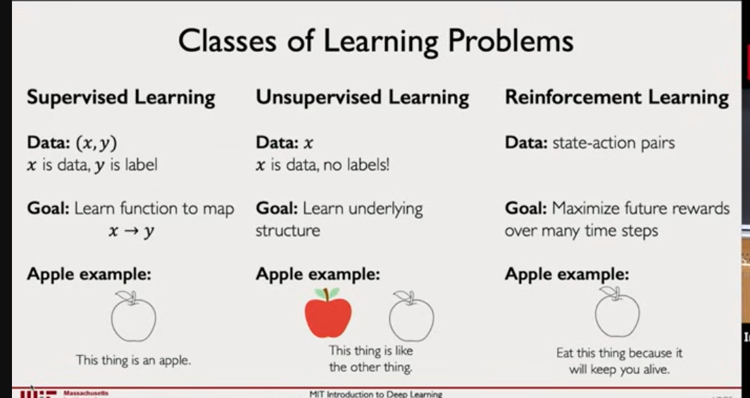
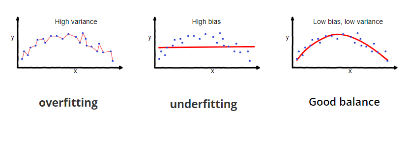
Bias and variance

Bias = how wrong the model’s assumptions are.

• Bias is error from wrong assumptions in the model.
  It measures how far the model’s average predictions are from the true values.
• High bias example: Using a straight line to fit curved data → model is too simple.

Variance = how unstable the model is to new data.

• Variance is error from sensitivity to training data.
  It measures how much the model’s predictions change if you train on different datasets.
• High variance example: A very deep decision tree that memorizes training data.
• Effect: Training error is low, but test error is high (overfitting).

Cross validation

Cross-validation is a technique where we split the dataset multiple times in different ways to test the model fairly.

The most common is k-Fold Cross Validation:

1. Divide data into k equal parts (called folds).
   Example: if k=5, split data into 5 parts.
2. Use 4 folds for training, and 1 fold for testing.
3. Repeat this k times, each time using a different fold as test.
4. Average the results → gives a more stable estimate of model performance.

Types of Cross-Validation

1. k-Fold CV → Most common (k=5 or 10 usually).
2. Stratified k-Fold → Ensures class proportions are same in each fold (good for classification).
3. Leave-One-Out (LOO) → Each data point is its own test set (expensive).
4. Shuffle-Split → Random splits multiple times.

Supervised Learning

Notes

• Are continous

Regression

Regression tasks involve predicting a continuous value for each input data point. Examples include predicting house prices based on features like square footage and number of bedrooms, predicting stock prices based on historical data.

• Ordinal Regression
• Linear Regression

Key Components:

1. Dependent Variable (Y): Same as in simple regression, this is the variable being predicted or explained.
2. Independent Variables (X₁, X₂, … Xₙ): These are the variables used to make predictions.
3. Regression Equation: The formula expands to accommodate multiple predictors: Y = β₀ + β₁X₁ + β₂X₂ + … + βₙXₙ + ε, where each β represents the coefficient for the corresponding independent variable.
4. Graph: In multiple linear regression, where there are multiple independent variables, the relationship is still linear, but the graph may not be a straight line in the traditional sense. Instead, it represents a hyperplane (A hyperplane is an (n-1)-dimensional subset of an n-dimensional space, dividing it into two distinct regions) in higher dimensions.

Assumptions of Linear Regression:

1. Linearity : The relationship between independent variable(s) X and dependent variable y should be linear (straight-line in 2D, hyperplane in higher dimensions).

2. Independence: Each observation should be independent. No data point should depend on another. If points are dependent, standard errors and significance tests become invalid.Suppose you collect students’ test scores, but you include the same student twice (before and after tutoring) as if they were independent. Their errors will be correlated (not independent).

3. Homoscedasticity: When we fit regression: $y={\beta }_0+{\beta }_{1}x+ϵ$

   • Residual ($ϵ$) = how far each actual $y$ is from the regression line.
   • Homoscedasticity = all residuals have roughly the same spread (variance), no matter the value of $x$.
   • Heteroscedasticity = the spread of residuals changes as $x$ increases.

   Say we’re predicting student score (y) from study hours (x). $(x,y)=\{(1,52),(2,60),(3,66),(4,75)\}$

   Residuals (errors) might look like: $ϵ=\{+2,-3,+1,0\}$

   Here, notice:

   • All errors are small (around ±3),
   • No matter if $x=1$ or $x=4$, the size of the errors is similar.

   This is homoscedasticity → equal spread.

   Let say if the error was $ϵ=\{+1,-2,+3,+15\}$

   • When $x=1$ or $x=2$, errors are small (±2).
   • But when $x=4$, error explodes to +15.

   That means the variance of errors increases with x → the “cloud” of points spreads out more at higher $x$.

4. Normality of Residuals

   Residuals should follow a normal distribution (bell-shaped around zero). This assumption matters mostly for hypothesis testing and confidence intervals. The coefficient estimates themselves don’t need normality, but inference assumes it.

5. No Multicollinearity Independent variables shouldn’t be highly correlated with each other.If two predictors carry the same information, the model struggles to separate their effects. Coefficients become unstable (high variance).

We can do linear regression in two way

• Normal Equation where we just plug the vaule we get a equation of line there is not loss and prediction
• Ordinary Least Squares : where we feed the input and check the loss and adjust the equation

Normal equation

We are going to use some Linear Algebra concepts for finding the right weight and bias terms for our data.

$$\begin{array}{rl}w+b& =1\text{for }(1,1)\\ 2w+b& =2\text{for }(2,2)\\ 3w+b& =2\text{for }(3,2)\end{array}$$

Let say the weight and bias terms are w and b respectively. So we can write each data point (x, y) as :

$$\left[\begin{array}{cc}1& 1\\ 2& 1\\ 3& 1\end{array}\right]\left[\begin{array}{c}w\\ b\end{array}\right]=\left[\begin{array}{c}1\\ 2\\ 2\end{array}\right]$$

we can write the above equations as a system of equations using matrices as Xθ = Y where X is input / feature matrix, θ is matrix for unknowns and Y is the target matrix as:

$$X\Theta =Y$$

Great, Now all we need is to solve this system of equations and get the w and b terms.

Wait there’s a problem. We can’t solve the above system of equations because target matrix Y does not lie in the column space(The column space of X = all possible linear combinations of those columns.) of input matrix X. In simple terms, if we see the previous graph again then we can notice that our data points are not collinear i.e. they don’t lie on the line so and that’s why we can’t find the w and b for the above system of equations.

And if we think for a moment then it sounds right because in Linear Regression we fit a hypothesis to predict the target for some input with the least possible error. We do not intend to predict the exact target.

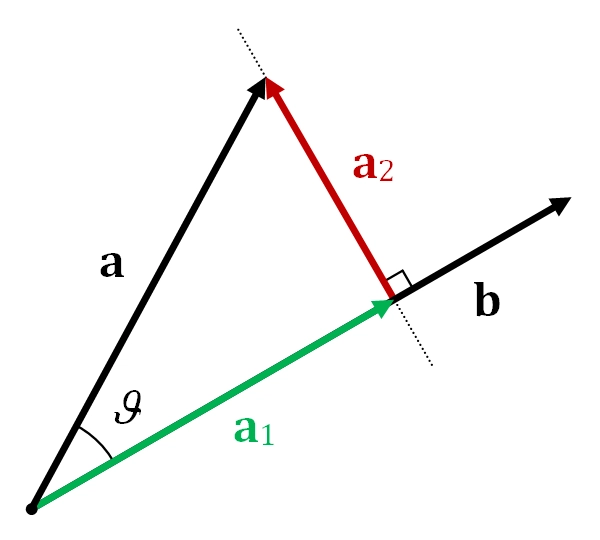
So what we can do here? We can’t solve the above system of equations because Y is not in the column space of X. So instead we can project the Y onto the column space of X. It is exactly equivalent to projecting one vector onto another.

In the above representation, a and b are two vectors and the a1 is the projection of vector a onto b. With this, we can see that now we have the component of vector a that lies in the vector space of b.

We can achieve the component of Y that lies in the column space of X by doing inner product (also known as dot product).

The inner product of two vectors a and b can be found by calculating aTb

Now we can re-write our system of equations as:
multiplying both sides by XT. Assuming (XTX) to be invertible

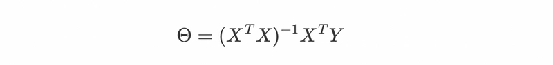
The above equation is known as Normal equation. Now we have the formula to find our matrix θ, let’s use it and calculate the w and b.

from the above last equation we have our w = 0.5 and b = 2/3 (0.6667) and we can check from the equation of blue line that our w and b are exactly correct. That’s how we can get the weights and bias terms for our perfect hypothesis using the Normal equation.

Ordinary Least Squares (OLS)

Log Regression

For classification loss function

• entrophy

confusion matrix → we use this to calculate accuracy , precisin,f1 etc

Polynomial Regression

Extends linear regression by adding powers of inputs: $y=w_0+w_{1}x+w_2{x}^2+w_3{x}^3+\dots$

• Captures curves instead of just straight lines.
• Example: Predicting growth rate of bacteria (which often follows a curved pattern).

Regularization

Regularization is a set of methods for reducing overfitting in machine learning models. Typically, regularization trades a marginal decrease in training accuracy for an increase in generalizability.

Let say we have model where we have trained using data and MSE (mean squred error) is very less now we have testing with test data where MSE is huge which is model is overfitting. so to avoid that we use regularization

Common methods:

1. Weight decay (L2)
2. L1 regularization
3. Dropout
4. Early stopping
5. Data augmentation
6. Batch norm
7. Smaller models
8. Noise injection
9. Label smoothing

In overfitting the MSE is very less so we add constant to our MSE equation to make the slope not ovefiting or underfiting

Ridge (L2) Regression

L2 regularization element is represented by the highlighted part. “Squared magnitude” of coefficient as penalty term is added to the loss function by ridge regression.

our goal is to make the weight small as possibel so we add sumation of all weight to our loss function such that if weight go up the loss will increase and the weight will decrease by our gradient due to heavy loss

$$\text{Loss}=\sum (y_i-{\hat{y}}_i{)}^2+\lambda \sum w_j^2$$

We add extra weight (that is slope) and lambda

Shrinks, keeps all. Best when all features are somewhat relevant.

Ridge (L1) Regression

L1 is smae as above but here we do absolute value of weight

$$\text{Loss}=\sum (y_i-{\hat{y}}_i{)}^2+\lambda \sum abs(w_j^2)$$

Same where we add magnitude of the weight.Shrinks AND kills some. Best when only a few features matter.

• Ridge (L2): penalty region is a circle (or sphere in higher dimensions).
• Lasso (L1): penalty region is a diamond (sharp corners at axes).

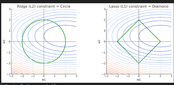
“What happens if we choose w1 and w2 to be different combinations of numbers?”

• w1 = first weight
• w2 = second weight

The graph is showing the space of all possible values of the two weights together.

This green shape represents:

“All weight combinations that satisfy the regularization limit.”

For L2 (Ridge) — the shape is a circle

Why?
L2 penalty = w1^2 + w2

All points with the same “size” lie on a circle.

For L1 (Lasso) — the shape is a diamond

Why?
L1 penalty = ∣w1∣+∣w2∣ All points with the same “size” form a diamond.

This is NOT about geometry — it is the shape of the constraint region created by the penalty.

Why large weights is problem

Large weights create extremely sharp boundaries When weights are large:

• A tiny shift in the input makes a huge change in the output.
• The model becomes unstable.
• It shapes extremely narrow, sharp patterns that perfectly carve around each training example.

This is exactly how memorization happens.

Data agumentation

Data augmentation is a technique used in machine learning and deep learning to artificially increase the size of a training dataset by generating new data from the existing data. This is typically done by applying random transformations (like rotations, translations, flipping, etc.) to the original data, creating slightly modified versions of the data that still retain the important features.

Common Data Augmentation Techniques:

1. Image Data Augmentation:
   • Rotation: Randomly rotating images by a certain degree (e.g., 90 degrees).
   • Flipping: Flipping images horizontally or vertically.
   • Translation: Shifting the image by a certain number of pixels in any direction.
   • Zooming: Randomly zooming into the image.
   • Shearing: Applying geometric transformations to the image to change the angles.
   • Brightness/Contrast adjustment: Varying the image’s brightness or contrast.
2. Text Data Augmentation:
   • Synonym replacement: Replacing words with their synonyms to create different sentences with similar meanings.
   • Random insertion: Inserting random words from a predefined list into sentences.
   • Back translation: Translating a sentence to a different language and then back to the original language to generate new variations.
3. Audio Data Augmentation:
   • Time stretching: Stretching or compressing the audio signal without changing its pitch.
   • Pitch shifting: Changing the pitch of the audio while preserving its speed.
   • Noise injection: Adding noise to the audio to make it more robust to background interference.

Classification

In classification tasks, the algorithm predicts a categorical label or class for each input data point. Examples include spam detection (classifying emails as spam or not spam)

• Binary Classification
• Multi-class Classification

Support vector machine

We want a machine that separates two groups of data (say cats vs dogs, spam vs not-spam, etc.) as well as possible.

• A line in 2D (or a plane in higher dimensions) can separate classes.
• Many such separating lines may exist — which one should we pick?

The Margin

Instead of just any separating line, SVM says:

Choose the line that leaves the widest possible gap between the two classes.

Support Vectors

Not all data points matter for drawing this “optimal” line.

• Only the points that sit right on the edge of the margin matter.
• These are called support vectors.
• They “hold up” the margin, just like tent poles hold up a tent.
  Move one, and the boundary shifts.

Nonlinear Boundaries

What if the data isn’t separable by a straight line?

SVM’s trick:

• Map the data into a higher-dimensional space where it is separable by a line.
• Example: Two concentric circles in 2D can’t be separated by a line in 2D, but if we map them into 3D cleverly, a flat plane can separate them.

This is called the kernel trick:

You don’t compute the high-dimensional mapping explicitly. Instead, you define a kernel function that measures similarity in that hidden space.

Soft Margins (Handling Mistakes)

In real life, data is noisy → perfect separation may be impossible.

SVM introduces a soft margin:

• Allow a few points to be misclassified.
• Still aim for a wide margin, but don’t obsess over fitting every noisy point.
• A parameter CC controls the tradeoff between:
  • Having a wider margin
  • Correctly classifying all training points

SVM Math

Step 1: Equation of a Straight Line

we already know slope-intercept form: $y=mx+b$

• $m$ = slope (how steep the line is).

If $m=2$, then every step in $x$ adds 2 steps in $y$.

• $b$ = intercept (where the line cuts the y-axis).

Example: $y=0.5x+1$.

• Intercept = 1 (when $x=0,y=1$).
• Slope = 0.5 (move right by 1 → go up 0.5).

Step 2: Problem with Vertical Lines

What if the line is vertical (like $x=4$)?

The slope-intercept form breaks (slope → ∞).

So we need a more general way.

Step 3: General Form of a Line

We can write a line as: $ax+by+c=0$

• $a,b$ = coefficients (decide the tilt of the line).
• $c$ = constant (shifts line up/down or left/right).

Example:

Convert $y=0.5x+1$ into general form: $0.5x-y+1=0$

Here:

• $a=0.5$,
• $b=-1$,
• $c=1$. This general form can also represent vertical lines (e.g. $x=4$ is just $1\cdot x+0\cdot y-4=0$).

Step 4: Which Side of the Line?

If you plug a point $(x,y)$ into $ax+by+c$:

• Result > 0 → point is on one side,
• Result < 0 → point is on the other side,
• Result = 0 → point lies exactly on the line.

Example: $0.5x-y+1=0$.

• Point (0,0): $0.5(0)-0+1=1>0$ → above line.
• Point (2,2): $0.5(2)-2+1=0$ → lies on line.

This is super important, because later SVMs use this test to classify points.

Step 5: Distance from a Point to a Line

Shortest distance formula:

$$\text{distance}=\frac{|ax+by+c|}{\sqrt{a^2+b^2}}$$

Example: line $x+y-4=0$, point (0,0).

Distance = $\frac{|0+0-4|}{\sqrt{1^2+1^2}}=\frac{4}{\sqrt{2}}=2.828$.

This gives the “gap” between the point and the line.

Step 6: Parallel Lines and Margin

If we shift the constant term:

$$ax+by+c=+1\text{(one line)}$$ $$ax+by+c=-1\text{(another line)}$$

These are parallel, equally spaced.

The gap (margin) between them:

$$\text{margin}=\frac{2}{\sqrt{a^2+b^2}}$$

This is the magic formula for margin width.

Step 7: Enter Support Vector Machines

Now, classification problem:

• Suppose yellow points = sick patients,
• Green points = healthy patients.

We want a line (hyperplane in higher dimensions) that separates them.

But there are infinitely many separating lines.

SVM’s trick: Pick the one with the biggest margin.

Why?

• Big margin = more “buffer space” = better generalization.

• The line is less sensitive to small changes in data.

Step 8: Support Vectors

Only the closest points (those lying on the margin lines) matter. They “support” the decision boundary. Move them → the boundary changes. All other points farther away are irrelevant.

Step 9: Standard SVM Formulation

We want:

• Maximize margin = Maximize $\frac{2}{\Vert w\Vert }$. (where $w=(a,b)$).
• Equivalently, minimize $\Vert w{\Vert }^2$.

Constraints: every point must be on correct side of margin:

$$y_i(w\cdot x_i+b)\ge 1\forall i$$

(where $y_i=+1$ for one class, $y_i=-1$ for the other).

So the optimization problem is:

$$\min \frac{1}{2}\Vert w{\Vert }^2\text{such that }{y}_i(w\cdot x_i+b)\ge 1$$

Step 10: Soft Margin (Noisy Data)

If perfect separation is impossible:

• Introduce slack variables ${\xi }_i$.
• Allow some points inside the margin or misclassified.

New problem:

$$\min \frac{1}{2}\Vert w{\Vert }^2+C\sum {\xi }_i$$

subject to:

$$y_i(w\cdot x_i+b)\ge 1-{\xi }_i,{\xi }_i\ge 0$$

Here, $C$ controls trade-off between wide margin vs fewer misclassifications.

Step 11: Kernels (Nonlinear Boundaries)

Sometimes data is not linearly separable.

SVM uses the kernel trick:

• Map data into higher dimensions,

• Then separate with a hyperplane there,

• Which corresponds to curved boundary in original space.

Example:

Data arranged in circles. Not separable in 2D.

But map $(x,y)$ to $(x^2+y^2)$ → becomes separable.

https://www.youtube.com/watch?v=gUzEN2TxnxE (SVM)

Decision Trees

A decision tree is a flowchart-like model that asks a sequence of questions about features and routes each example down a path until a leaf node gives the prediction. Each internal node tests a single feature (categorical test or numeric threshold). Leaves contain predictions (class label or numeric value).

• Root node: top-most node.
• Internal node (branch): a non-leaf node with a test & child nodes.
• Leaf node (terminal): no children; contains prediction.
• Pure node: all training examples in the node share same class.
• Impurity: measure of how mixed a node is.

Types

• Classification tree → leaf outputs a class (e.g., Yes / No).
• Regression tree → leaf outputs a numeric value (usually the mean of targets in that leaf).

To train a Decision Tree from data means to figure out the order in which the decisions should be assembled from the root to the leaves. New data may then be passed from the top down until reaching a leaf node, representing a prediction for that data point.

Entropy

The entropy function measures the uncertainty or disorder in the set of events. If the probabilities of all events are equal (e.g., for a fair die), the uncertainty is the highest, since you have no idea which specific outcome will occur.

Conversely, if one outcome is certain (e.g., p1=1 and all others are zero), there is no uncertainty (i.e., entropy is zero).

$$H=-\sum _{i=1}^n{p}_i{\log }_2(p_i)$$

Where:

• $H$ is the entropy (the measure of uncertainty or disorder).
• $n$ is the number of different possible events or outcomes.
• $p_i$ is the probability of the $i^{th}$ event (it’s the likelihood of each outcome occurring).
• ${\log }_2(p_i)$ is the logarithm base 2 of the probability $p_i$.

• The logarithmic function comes from information theory and quantifies the amount of information produced by an event.
  • If an event has a high probability (close to 1), it provides less information (it’s more predictable). On the other hand, if an event has a low probability (close to 0), it provides more information because it’s more surprising.
  • Logarithms help normalize the scale of information: events with higher probabilities contribute less to the entropy, while rare events contribute more.
• The Negative Sign:
  • The negative sign is needed because the logarithm of a probability (which is less than 1) is negative, and we want entropy to be a positive value.
  • In essence, entropy is a positive quantity that quantifies disorder or uncertainty.

The range of entropy values:

• Minimum entropy: $H=0$ (perfect certainty, no uncertainty)
• Maximum entropy: $H={\log }_2(n)$, where $n$ is the number of possible outcomes, representing maximum uncertainty.

Information Gain

The information gain measures how much the entropy (uncertainty) is reduced by splitting the data on feature A. If splitting the data on A significantly reduces the uncertainty about the target class, the information gain will be high.

• If Information Gain is high: The feature AAA has a strong ability to classify the data and reduce uncertainty.

• If Information Gain is low: The feature AAA does not provide much information about the target class.

Algorithms to gain information gain

Algorithm	Split Criterion	Handles Continuous?	Typical Splits	Notes
ID3	Entropy / Information Gain	No (originally)	Multiway	Simple, but biased to many categories
C4.5	Gain Ratio	Yes	Multiway	Fixes ID3, adds pruning
CART	Gini (classification), Variance (regression)	Yes	Binary	Most widely used
CHAID	Chi-square test	Yes	Multiway	Popular in marketing, stats-heavy

Gini impurity

Gini impurity measures how “mixed up” a set of items is. Another way to think about it:

If I randomly pick two items from this set, how likely are they to be of different classes?

The more often you get different classes, the more impure the set is.

Let say we have two color of socks where have put in a box where we have red color 7 and blue color 3 so we need to find the probablity of picking two times that will from differenet color socks that is first time red and blue if we have high probablity mean we have impure the data is not pure

Suppose we have two classes, Red and Blue.

• Let $p_{\text{red}}$ = probability of picking a red sock
• Let $p_{\text{blue}}$ = probability of picking a blue sock = $1-p_{\text{red}}$

If you pick two socks randomly, there are four equally likely “ordered outcomes”:

1. Red then Red → probability $p_{\text{red}}\cdot p_{\text{red}}=p_{\text{red}}^2$
2. Red then Blue → probability $p_{\text{red}}\cdot p_{\text{blue}}$
3. Blue then Red → probability $p_{\text{blue}}\cdot p_{\text{red}}$
4. Blue then Blue → probability $p_{\text{blue}}^2$

The probability that the two socks are different colors = cases 2 + 3 =

$p_{\text{red}}\cdot p_{\text{blue}}+p_{\text{blue}}\cdot p_{\text{red}}=2p_{\text{red}}{p}_{\text{blue}}$

The probability that the two socks are the same color = cases 1 + 4 = $p_{\text{red}}^2+p_{\text{blue}}^2$

Notice that:$1-(p_{\text{red}}^2+p_{\text{blue}}^2)=1-p_{\text{red}}^2-p_{\text{blue}}^2$

If you expand $(p_{\text{red}}+p_{\text{blue}}{)}^2$: $(p_{\text{red}}+p_{\text{blue}}{)}^2=p_{\text{red}}^2+2p_{\text{red}}{p}_{\text{blue}}+p_{\text{blue}}^2=1$

So: $2p_{\text{red}}{p}_{\text{blue}}=1-(p_{\text{red}}^2+p_{\text{blue}}^2)$

Exactly the Gini formula!

Gini impurity is a measure of how “mixed up” a set of items is.

• If all items are the same class → perfectly pure → Gini = 0
• If items are evenly mixed → very impure → Gini close to maximum

We need a numerical way to measure this impurity.

Note:

• Gini: If I randomly grab two socks, how often do I get a different color?
• Entropy: If I randomly grab one sock, how unsure am I about its color?

Random Forests

 Naive Bayes

It helps us to tell what is the probablity of A happens on B

example: we get 90% car get accident what is probality of this car get accident

$P(A|B)=\frac{P(A\cap B)}{P(B)}$

in real life we not able to find A intersection B so we did some subsition and math we get

$P(A\mid B)=\frac{P(B\mid A)\times P(A)}{P(B)}$

Symbol	Meaning	Intuition
(P(A))	Prior	How likely (A) was before we saw (B).
(P(B \mid A))	Likelihood	How consistent (B) is with (A) being true.
(P(B))	Evidence (normalizer)	How often (B) happens overall.
(P(A \mid B))	Posterior	Our updated belief in (A) after seeing (B).
it’s just the conditional probability definition rewritten to express it in a more useful form.

Example let say we have alram in house and it will on when the unknow preson enter to the home

let we have 1000 houese and we hearing the alram what is probablity of that alram is due to some unknow person enter to home

burglary → a unknown person enter to house

• Alarms are 90% reliable — they go off when a burglary happens.
  → P(alarm | burglary)=0.9

• But sometimes, they false-alarm (maybe cat triggers it):
  → P(alarm | no burglary)=0.1

• And in your town, only 1 house in 1000 gets burgled.
  → P(burglary)=0.001

Case	Houses	Alarm triggers?	Count of alarms
Burglary	1	90% of time	0.9 alarms
No burglary	999	10% of time (false alarm)	99.9 alarms

Term	Meaning	Value
P(A)	Prior unknow person chance	0.001
P(B \mid A)	Alarm goes off during burglary	0.9
P(B)	Any alarm going off	0.1008

P(burglary | alarm)=0.9/100.8≈0.009

That’s less than 1%.

Even though the alarm is 90% accurate,
because burglaries are so rare, most alarms are still false.

The alarm isn’t lying — it’s just that false alarms happen way more often than real burglaries.

Your brain’s natural mistake is to focus only on the “90% reliable” part and forget the base rate (how rare burglaries actually are).

Bayes’ theorem corrects that mistake mathematically.
It says:

“Don’t just look at how accurate the clue is — also weigh how common each cause is.”

That’s all Bayes does.

Ensemble Learning

Ensemble learning is a technique in machine learning where we don’t rely on just one model, but instead combine multiple models to make better predictions.

Types of Ensemble Learning

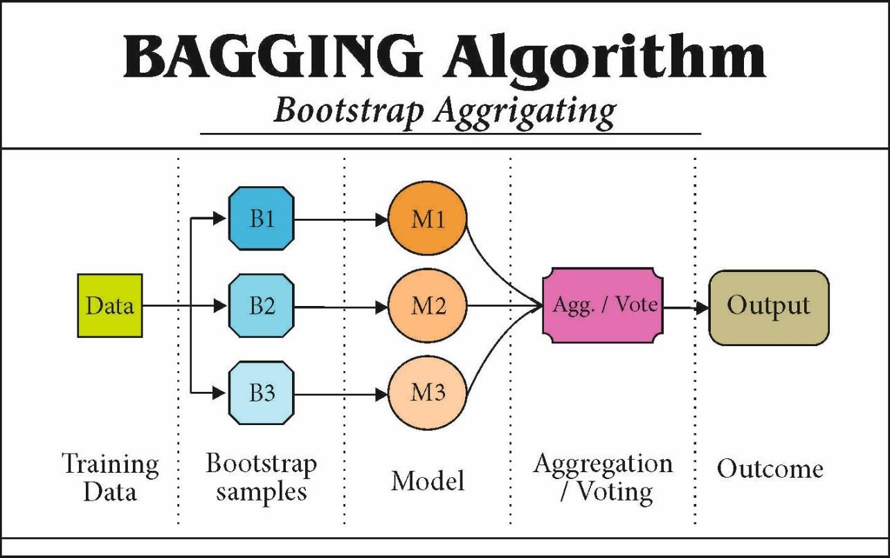
Bagging (Bootstrap Aggregating) Train multiple models (usually of the same type, like decision trees) on different random subsets of the training data. Combine their predictions (by averaging for regression, or majority vote for classification). Example: Random Forest.

Bootstrap samples Bootstrap = “resample with replacement.”

• we have an original dataset with, say, 100 training points.
• To make a bootstrap sample, you randomly pick 100 points with replacement.

With replacement means: after picking one point, we put it back before picking the next. So some points may appear multiple times, and some may be missing. Example:

• Original dataset = {A, B, C, D}
• One bootstrap sample could be {B, C, C, A} This way, each bootstrap sample is slightly different, like giving each model a different perspective of the data.

Aggregate

• For classification → take a majority vote
• For regression → take the average prediction

Boosting

• Train models sequentially, each one trying to fix the mistakes of the previous one.
• Combine them with weighted votes.
• Examples: AdaBoost, Gradient Boosting, XGBoost, LightGBM, CatBoost.

Stacking

• Train multiple models (can be different types) in parallel.
• Then use another model (a “meta-learner”) to combine their predictions.

Workflow

Data → Feature Representation → Model Family → Parameters → Prediction Function → Loss → Optimization → Regularization → Training Procedure → Evaluation → Inference

Data Collection → Data Validation → Feature Representation → 
Feature Selection → Model Family Selection → Hyperparameter Tuning → 
Model Parameters → Prediction Function → Loss Function → 
Optimization → Regularization → Training Procedure → 
Evaluation → Error Analysis → Explainability & Interpretability → 
Inference → Model Monitoring & Drift Detection → [Loop back for Retraining]

Input Representation

How raw data is turned into features.

• Example: Bag of Words for text, pixels for images, embeddings, etc.

Model (Hypothesis Class)

The family of functions the algorithm can choose from.

• Linear models, decision trees, neural networks, SVMs, etc.

Parameters

The adjustable numbers inside the model.

• Example: weights www and bias bbb in linear models; millions of parameters in deep nets.

Prediction Function

How the model maps input features → outputs.

• Example: $\hat{y}=w\cdot x+b$ (linear regression)
• Example: $\hat{y}=\text{softmax}(Wx+b)$ (classification NN)

Loss (or Cost) Function

A function that measures how far predictions are from truth.

• Regression: Mean Squared Error (MSE)
• Classification: Cross-Entropy Loss
• SVM: Hinge Loss

Optimization Algorithm

The method for adjusting parameters to minimize loss.

• Gradient Descent, SGD, Adam, etc.

Regularization

Extra terms to prevent overfitting.

• L1, L2 penalties, dropout, early stopping.

Training Procedure

Rules for how to present data and update parameters.

• Batch size, number of epochs, learning rate schedule.

Evaluation Metric

Loss is used during training. But we also need separate metrics to judge performance.

• Accuracy, Precision/Recall, F1-score, AUC, RMSE, etc.

Name	Description	Loss Function	Type	Optimization	Regularization	Key Hyperparameters	Assumptions	Pros	Cons	Typical Use Cases
Linear Regression	Predicts continuous output using linear combination of inputs	MSE	Regression	Gradient Descent, Normal Equation	L1, L2	Learning rate, regularization strength	Linearity, independent errors, homoscedasticity	Simple, interpretable	Sensitive to outliers, cannot capture non-linearity	Predicting prices, trends
Logistic Regression	Models probability of binary outcome using sigmoid	Binary Cross-Entropy	Classification	Gradient Descent, LBFGS	L1, L2	Learning rate, regularization	Linearity in log-odds, independent features	Interpretable, fast	Cannot handle complex non-linear relationships	Spam detection, medical diagnosis
Decision Tree	Splits data into branches based on features	Gini, Entropy, MSE	Both	Greedy recursive splitting	Max depth, min samples	Max depth, min samples per leaf	No strong assumptions	Interpretable, handles non-linear	Prone to overfitting	Classification/regression on tabular data
Random Forest	Ensemble of decision trees using bagging	Same as DT	Both	Greedy splitting per tree	Max depth, min samples, feature subsampling	Number of trees, max features	Trees are independent	Reduces overfitting, robust	Less interpretable, memory intensive	Predictive modeling on tabular data
XGBoost	Gradient boosting of trees sequentially	Log Loss, MSE	Both	Gradient Boosting, Newton-Raphson	L1, L2, tree pruning	Learning rate, n_estimators, max_depth	Weak learner assumption	High performance, handles missing data	Complex tuning, less interpretable	Kaggle competitions, structured data
SVM	Finds optimal hyperplane for separation	Hinge (classification), Epsilon-insensitive (regression)	Both	Quadratic Programming, SGD	C parameter (margin), kernel choice	Kernel type, C, gamma	Linearly separable in kernel space	Effective in high dimensions	Not scalable to huge datasets	Text classification, image recognition
K-Nearest Neighbors	Predicts based on neighbors	Distance-based	Both	Lazy learning (no optimization)	None	k, distance metric	Assumes similar points are close	Simple, non-parametric	Slow for large datasets, sensitive to noise	Recommender systems, anomaly detection
Naive Bayes	Probabilistic classifier assuming feature independence	Negative log-likelihood	Classification	Maximum Likelihood Estimation	None	Prior type, smoothing	Feature independence	Fast, works with small data	Oversimplified assumptions	Text classification, spam filtering
k-Means	Partitions data into k clusters	Sum of squared distances	Unsupervised	Lloyd’s Algorithm (iterative)	None	Number of clusters k, init method	Spherical clusters, equal variance	Simple, scalable	Sensitive to initialization, non-convex clusters	Customer segmentation, clustering
Hierarchical Clustering	Builds tree of clusters	Linkage-based distance	Unsupervised	Agglomerative / Divisive	None	Linkage type, distance metric	Assumes meaningful hierarchical structure	Dendrogram interpretable	Computationally expensive	Taxonomy, gene clustering
PCA	Dimensionality reduction via orthogonal projection	Reconstruction error	Unsupervised / Feature Extraction	Eigen decomposition, SVD	None	Number of components	Linearity, large variance = important	Reduces dimensionality	Loses interpretability	Visualization, feature compression
LDA	Projects data to maximize class separability	Log-likelihood	Classification / Dimensionality Reduction	Eigen decomposition	None	Number of components	Normality, equal covariance	Good for separable classes	Not for non-linear boundaries	Face recognition, classification
GBM	Sequential ensemble to reduce error	MSE, Log Loss	Both	Gradient Boosting	L1, L2	Learning rate, n_estimators, max_depth	Weak learner assumption	High accuracy	Slower, complex tuning	Structured tabular prediction
AdaBoost	Focuses on misclassified points sequentially	Exponential loss	Both	Stage-wise additive modeling	None	Number of estimators, learning rate	Weak learners	Reduces bias	Sensitive to noisy data	Classification tasks
Neural Networks (MLP)	Layered neurons for non-linear mappings	MSE, Cross-Entropy	Both	SGD, Adam, RMSProp	L1, L2, Dropout	Layers, nodes, activation, learning rate	Large data required	Flexible, handles complex patterns	Hard to interpret, tuning heavy	Image, text, tabular data
CNN	Specialized for image/spatial data	Cross-Entropy, MSE	Both	SGD, Adam	L2, Dropout, BatchNorm	Filters, layers, stride	Spatial invariance	Excellent for images	Data hungry, computational	Image recognition, segmentation
RNN / LSTM	Sequence modeling	Cross-Entropy, MSE	Both	SGD, Adam	L2, Dropout	Hidden units, timesteps, layers	Sequential dependencies	Captures temporal info	Vanishing gradients, slow	Time series, NLP
Autoencoders	Unsupervised feature learning	Reconstruction loss	Unsupervised	SGD, Adam	L2, Dropout	Layers, bottleneck size	Data manifold structure	Dimensionality reduction	Can overfit	Anomaly detection, compression
GMM	Probabilistic model with Gaussian mixtures	Log-likelihood	Unsupervised / Clustering	EM Algorithm	None	Number of components, init	Gaussian distribution	Soft clustering, flexible	Sensitive to initialization	Clustering, density estimation
Reinforcement Learning	Learns policy to maximize reward	TD loss, Policy gradient	RL	Q-Learning, Policy Gradients	None	Learning rate, gamma, epsilon	Markov Decision Process	Optimizes sequential decisions	Sample inefficient, complex	Game AI, robotics
DBSCAN	Density-based clustering	Density-reachability	Unsupervised	DBSCAN algorithm	None	Epsilon, min_samples	Varies density clusters	Finds arbitrary shape clusters	Fails with varying densities	Anomaly detection, spatial data
CatBoost	Gradient boosting for categorical data	Log Loss, RMSE	Both	Gradient Boosting	L2, leaf-wise	Learning rate, depth, iterations	Weak learner assumption	Handles categorical natively	Complex tuning	Tabular data with categories
LightGBM	Gradient boosting optimized for speed/memory	Customizable	Both	Gradient Boosting	L2, leaf-wise	Learning rate, num_leaves, boosting type	Weak learner assumption	Fast, scalable	Sensitive to overfitting	Large-scale tabular data

UnSupervised Learning

perceptron

AutoML

Frameworks represent a noteworthy leap in the evolution of machine learning. By streamlining the complete model development cycle, including tasks such as data cleaning, feature selection, model training, and hyperparameter tuning, AutoML frameworks significantly economize on the time and effort customarily expended by data scientists.

Feature engineering

process of creating new features or transforming existing features in a dataset to improve the performance of machine learning models. It involves selecting, extracting, and transforming raw data into meaningful features that can help the model better understand the underlying patterns in the data.

for more Feature Engineering

Model performance assessment metrics

Confusion Matrix: A confusion matrix is a table that is often used to describe the performance of a classification model on a set of test data for which the true values are known. It consists of four elements:

• True Positive (TP): The number of instances correctly predicted as positive.
• True Negative (TN): The number of instances correctly predicted as negative.
• False Positive (FP): Also known as Type I error, the number of instances incorrectly predicted as positive.
• False Negative (FN): Also known as Type II error, the number of instances incorrectly predicted as negative. A confusion matrix provides insights into the performance of a classification model and can be used to calculate various metrics such as accuracy, precision, recall, and F1-score.

Accuracy: Accuracy is the ratio of correctly predicted instances to the total number of instances in the dataset. It is calculated as:

Accuracy= TP + TN / TP + TN +FP +FN​

Cost-Sensitive Accuracy: Cost-sensitive accuracy takes into account the costs associated with different types of errors. It assigns different weights or costs to different types of errors based on their importance. For example, in medical diagnosis, the cost of false negatives (missed diagnoses) might be much higher than the cost of false positives (incorrect diagnoses). Cost-sensitive accuracy is calculated by adjusting the weights of TP, TN, FP, and FN accordingly.

Precision: Precision is the ratio of correctly predicted positive instances to the total number of instances predicted as positive.

	Precision = TP / TP + FP

Recall (Sensitivity): Recall, also known as sensitivity or true positive rate, is the ratio of correctly predicted positive instances to the total number of actual positive instances.

Recall=TP / TP + FN

F1-Score: F1-score is the harmonic mean of precision and recall. It balances precision and recall and provides a single metric that summarizes the performance of a classifier.

F1_score = 2* Precision * recall / Precision + recall 

Resources

• ML system design: 450 case studies to learn from
• https://distill.pub/
• https://dafriedman97.github.io/mlbook/content/introduction.html
• MLSys Seminars
• https://ocdevel.com/blog
• Best machine learning self-taught resources in 2025
• https://medium.com/@sundharesansk11/understanding-linear-regression-with-ordinary-least-squares-a7fd6e2052fb
• MLU is an education initiative from Amazon designed to teach machine learning theory and practical application.
• https://developers.google.com/machine-learning/guides/rules-of-ml

Best

• Learn how to combine machine learning with software engineering to design, develop, deploy and iterate on production-grade ML applications.

Maths

• https://freedium.cfd/https://towardsdatascience.com/how-to-learn-math-for-machine-learning-fast-even-with-zero-math-background-159757833c3a